Revised January 2026
What did I do during the war that was Apartheid?
What did you do during the Apartheid years? It is a question that might be asked of my life in South Africa. My answers, believed or disbelieved, will have no practical consequence. I am very unlikely to be punished or rewarded for my past actions or for want of them. I sense that what people of my generation did during the apartheid years is of little interest to the current powers that be. I do not intend to apologise for what I did, or did not do, to make South Africa a better place than it was before it became a true democracy- which it is- and which I welcomed without reservations at the time. It came as a great relief and a welcome surprise.
Service to the old regime
I had served as a member of the SA government’s Competition Board between 1983 and 1989. I had also served as an advisor to the Margo Tax Commission in 1986. I was appointed to serve as the non-executive chairman of the Victoria and Alfred Waterfront Company in 1989, a newly established subsidiary of the State Owned Transport conglomerate, Transnet, that not too long before was known as South African Railways and Harbours. (SAR&H) They also ran the national airline carrier SAA.
The V&A was established to redevelop the historic harbour of Cape Town. Apparently, my appointment was confirmed at the highest levels of the Government of the much-reviled President P.W. Botha, the leader who refused to cross the Rubicon to majority rule in 1985. Eli Louw, then the Minister of Transport, whom I had once advised at his request on an exchange rate question asked of him in Parliament, had supported my appointment recommended as it was by the senior executives of Transnet.
The decision that made the Waterfront development possible was taken before I joined the project. A committee led by Arrie Burggraaf, a senior harbour engineer, had decided that the development need not prejudice the workings of the commercial harbour, then largely a fishing port. Which it has not done and fishing remains an important activity in the old Victorian Basin. Indeed the still working harbour adds intended authenticity and interest to the recreational and shopping activities that were added to the much redeveloped site. Arrie continued to serve the project most ably as a director. Rudi Basson who ran the harbour at the time was highly supportive of our venture- an indispensable ingredient for its early progress.
Mike Myburgh who ran SA Airways, at the time also part of Transnet and Fuzz Loubser from the Property division, who had participated in a course for practicing executives in the property sector held at the UCT Graduate School of Business on which I had lectured, approached me to accept the appointment as non-executive chairman. At R30000 a year in 1988, a stipend that had remained unchanged 13 years later in 2001 after the CPI had increased by about five times, when I was asked to hand over to those more empowered.
I didn’t ask and I was not offered any inflation adjustment- perhaps an indicator of poor negotiating skills. And there were no additional payments for attending the many meetings or the like as seems to be custom of the many agencies with a public purpose. As I like to say not for profits, only for employment benefits. The success of the project was ample reward for my efforts.
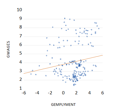
The Transnet innovators were very keen to present the Waterfront project as a private rather than a public enterprise. And they thought I could give it some private sector credentials. The conversion of the V&A Waterfront to a privately-owned company, as was the original intention, came after my time with it. I would have liked to have led the conversion of the company to a stand-alone and listed entity on the Johannesburg Stock exchange which would have been highly possible as its development to date proves. There is an extensive literature on the Waterfront and its development. [1]
It was an appointment I welcomed and a role I pursued as vigorously as I knew how. The success of the project would be very good for Cape Town, as I hoped and thought it would be, at that most difficult time for the economy. Yet many opponents of South Africa as it was, did not wish us well. A stronger economy improved the survival prospects of white rule, which undoubtedly it did – all else remaining the same- which clearly did not. But a stronger economy also meant less poverty as I saw it and if I could contribute to poverty relief, I was happy to do so. The prospect of revolutionary change in SA at that time seemed very remote with or without a stronger economy.
Guilt by association
Yet by continuing to live in South Africa one was inevitably something of a collaborator in an evil system from which you benefitted or rather suffered very little. Even if you used whatever powers of persuasion and analysis to argue for something better than affirmative action for white South Africans. I did not approve of sanctions or boycotts against South Africa or my university or a violent insurrection. I was never a supporter of the ANC. I was an anti-communist much influenced by what I read in Encounter and Commentary magazines. Darkness at Noon by Arthur Koestler and Homage to Catalonia by George Orwell were very important testimonies for me. I regarded the Soviet Union as a very evil empire before Ronald Reagan pronounced it so. The work of Pasternak and later Solzhenitsyn confirmed my judgment. Communism was poor theory – it was horrific in practice.
That the ANC was funded and supported by the Soviets made it impossible for me to hope for their success. Moreover, I was always hopeful against hope that we could make South Africa a better place by reforming its economy, even if reforming its politics seemed much less likely. I always hoped for the best, tried to emphasize an upside rather than the opposite, and perhaps provided encouragement to others, those who like myself did not emigrate. My sharing a sense of the upside was one of the reasons my many speeches and presentations to business audiences were appreciated and generally welcomed. I was able to share some hope for the future that appeared so clouded. I was described as a serial optimist, not necessarily with approval. I am still one though with reservations about the new South Africa.
I worked with the government as a member of the Competition Board for six years in the mid-eighties believing that I was doing some good. And as an advisor to the Margo Tax Commission in 1986 with the same intentions. I had always hoped for the economic success of South Africa and still fervently do so, as I did of its sporting teams even though they represented only a minority of the population. I remain a highly enthusiastic supporter of South African sporting teams and individuals. I regard the transformation of the Springbok rugby team, that remains highly competitive, as a role model for South Africa.
Why me?
I was often asked somewhat disparagingly why they chose me to lead the Waterfront project given my obvious lack of knowledge or experience. I was reminded recently by our outstanding Managing Director David Jack, who was highly knowledgeable and experienced in matters of waterfront development, that in the meeting that introduced the project to a highly sceptical public, I had promised to “apply my mind”. Which I did, helped greatly by David, who turned out to be an outstandingly good appointment as managing director.
He was the City of Cape Town Planner at the time with excellent experience gained in waterfront development at Marina da Gama, when working for Anglo-American. The development of Mitchells Plain for the City of Cape Town was among his achievements.
Good relationships with the City that David could bring to the project, were a very important requirement for the success of our project. Being sponsored by the authority that ran and owned the harbour facilities gave us strength in the planning process that is not available to the ordinary developer. We were able to achieve flexibility in the approved development plan that proved very valuable in being able to respond to market demands for different uses of our land as they were revealed. We were thus able to flexibly respond to market trends. We were market rather than planning led. The results of our efforts is an asset that the new South Africa can be proud of and benefits from.
It was cricket
No normal business in an abnormal society might have been their slogan. As it was chanted in sport – “no normal sport in an abnormal society” the chant aimed at the members of the Green Point Cricket Club, when we successfully opened the club to all races in the mid-seventies. I was the hard-working Club Captain at the time looking after the eleven teams we fielded every Saturday (without the help of the mobile phone) when still an active cricketer. It was a bold move made without universal approval, as we were well-aware. A number of not-white cricketers of all competencies chose to accept our invitation to enjoy a better standard of cricket than was being offered them.
That we could open the club to all comers in what had been strictly racially exclusive sport was a sign of the changing times. We could not have managed without our chairman Gerald Mallinick, who was a keen, brave cricketer, he took many a catch fielding close in at short leg off my inswingers. But more important he was an even more determined lawyer. He and his impressive legal practice were strong defenders of justice for all. It would not have happened without Gerald. And all the members of the club welcomed its opening without any dissension at all. It was the right thing to do, and the club to its credit, was fully united in the step we took. Nor were we prevented or indeed discouraged from proceeding on our multi-racial course by our opponents on the field or the administrators. Times they were a’ changing.
The advantages of an excellent partner in life
I was a good citizen in a land that had turned in a badly wrong direction. I had a successful university and business career. I was able to support my family and be an attentive son for my parents who, who loved our boys, who that were growing up fast under their eyes. My folks lived interesting healthy and independent lives and held an extended loving wider family together until the end.
I was able to pay the school and reduced university fees for our boys Charles and Daniel who graduated in Economics and Law (a fringe benefit for all present and past employees of UCT – and also for professors-emeriti) And also pay reduced university fees for my wife of over 50 years now, Shirley who graduated as a Master of Fine Arts in 2002 and has been a dedicated registered student of English, Music and Language, who consistently achieves excellent marks for her essays and examinations. If only all students were as hard working and committed as she. Shirley is a remarkably determined woman with extraordinary physical strength and powers of concentration.
Her working life began with radiography. By sheer chance, she was on duty that fateful night at Groote Schuur hospital in November 1967, and took the X rays of Chris Barnard’s first heart transplant patient. Do ask her to tell her story of that early morning in the operating theatre? It is great theatre.
Besides bring up our two boys who were born in quick succession, Shirley taught art history to matriculants at the Cape Tec, and Chinese cooking to what was then a largely uninitiated but appreciative clientele in Cape Town. Doing so with success both financial and culinary. The extra income at the time was very welcome.
I used to return from trips to Johannesburg with dangerous looking cleavers and woks bought from a Chinese store in lower Commissioner Street that were sold on to her students. Nobody stopped me carrying them on board in my hand luggage. Hijacking only came later. And the two boys were on hand when she returned from those evenings of good food and good instruction, to help count the cash that spilled out from her apron.
Thereafter cooking gave way to making paper by hand on our lawn in Camps Bay to which we moved from Sea Point in 1985. We had sold and bought at the top of the housing boom- when house prices are adjusted for inflation. Her paper is beautifully crafted of which we have a fine collection. Then followed seven busy years as the curator of the Baxter Art Gallery at the Baxter Theatre of the University of Cape Town where what were to become famous and successful South African artists were first exhibited. Helen Sabidi, Willie Bester, Carol Boyes, Tyrone Appolis among them. Her next project was to establish her own NGO, the Arts Foundation that brought together many school children from all the diverse and still racially separated communities of Cape Town to enhance their creative senses and to meet each other, that was so difficult in those days. The venue for their immersion in the arts was the good ship RSA- the original SA voyager to the South Pole, that was laid up at the Waterfront. The Arts Foundation ended as the RSA started to sink and was buried in Table Bay. The BA and then MA in fine arts at the Michaelis Art School followed. Shirley has introduced me to and kept me well informed about the academic zeitgeist. I understand the world of art and literature much better for her influence. I am still receiving much insight and instruction from her.
The 24/7 Economist
Though I claim to be an expert only on economic life – and on cricket as all will be revealed. Some of the work I did with Graham Barr on trading off risk and returns on the cricket field was published in a leading Journal, that of the Operations Research Society as well as in the local Journal of Statistics. The version included below in the post-script is the one I wrote for our clients of Investec before the World Cup of 2007. We still receive many requests, naturally from cricket-mad India, for copies of the work we did.
I also wrote with my economist hat, always on, about restaurants, explaining why no one goes to the empty establishment and would prefer to wait in line at the busy venue. A sub-editors bye line in the article read “Empty tables are a restaurateur’s curse, not because they are empty, but because they keep customers out”
I explained why paying more for your wine means paying less for your food and vegetables, a case of convenient bundling, as practiced by any supermarket and in many other contexts. It is what you pay for the bundle, the trolley load not the tomatoes, that brings you back. I was intrigued also by the fact that in wine, unlike most goods and services you have two independent measures of quality. Price and the points scored by a wine at the wine tastings. I found that the correlation between the log of price and scores was positive and statistically significant but left ample room for a bargain. That is to pay less for a bottle than would have been predicted by its score. I was also able to satisfy myself in another study using the same method that South African wines are not underpriced for their quality as measured by their scores in international tastings. (Wine, April 1997 and below)
A final word in my own favour – on family and friends
Elder son Charles in New York since 1991 where he practices very successfully as a financial advisor and investor. He knows how to run a successful business managing other people’s money in the most competitive of markets, a skill he would not have learned from his father. Charles married Amy Bedrick from Providence, Rhode Island in 1997 and they are happily together. Their finest achievement has been to have brought up two remarkable and likable young women Abigail and Lindsey. Abigail has now graduated from Duke University with honours and is working in Washington and Lindsey is a fresher at Duke I have observed how good their schooling has been at Columbia Grammar School on the upper west side of Manhatten. Meeting the New York family but once or twice a year, and not since the pandemic reminds us how much is lost living so far apart.
Our younger son Daniel lives round the corner with his wife Kubesh and son Jody who a great joy to us. Daniel practices law and is a lively entrepreneur developing the local market for South African Olive Oil which deserves more respect and higher prices, as does our wine.
I have led a purposeful and mostly joyous life in the company of many agreeable friends in the pristine setting of Cape Town. Access to the mountain and the sea gave much pleasure over many years and still does so. I have no regrets at all that I did not seek fortune and influence elsewhere, especially now that all that past, deeply contaminated water has long flowed under the bridge. I did not emigrate as I might have done and thought often about doing. It turned out well that my boys did not have to serve in the army which would have meant emigration. The fight was over by the time they graduated.
With the hindsight now of twenty years spent as a full-time financial analyst and a part time academic rather than the other way round as it was, I am of the view that I could have succeeded financially in the USA or the UK at least as well as I have done in SA – had I entered the financial markets earlier. As an economist or investment strategist I believe, perhaps immodestly, that I would have been competitive. I like to say that it takes a good economist to recognize one. And that it is hard for the non-economist to recognize the difference which is part of the problem of proving anything in economics. I have had the good fortune to enjoy all too briefly the company of some of the best economists of my era, a number outside of SA when the opportunity was presented on sabbaticals or when attending conferences. I did not lack for the confidence that I could be in their company.
Giving comfort in addressing the SA upside
I enjoyed and was encouraged by some strong support from ex-students and readers and attenders of my talks and presentations listeners at home. My first attempts to reach a wider audience were published by the Cape Town Chamber of Commerce in their Commercial Opinion, well edited by Bill West, whom I remember with much appreciation as I do Brian McCloud, who ran the local Chamber at the time and helped me focus on business rather than government activity. One early article made the case for an expenditure rather than an income tax – promoted by Nicholas Kaldor a leading and very left-wing Cambridge economist.
I have always thought that it is better to tax individuals on what they take out of the economy, their consumption, rather than what they put into the economy as measured by their incomes. Kaldor had shown that a consumption tax could be made progressive by imputation from reported earnings and before and after balance sheets. Consumption funded by reducing a stock of wealth would then be included in the tax net with the consumption tax collected at the various tills credited as a withheld tax to be set off against the tax bill.
I used to regularly attend the meetings of the Chamber’s Economic Committee soon after being appointed as a Junior Lecturer. The economics department at UCT had been approached by the Chamber to second a faculty member to attend meetings of the Chamber. I happily attended meetings of the economic sub-committee regularly and took a keen interest in the deliberations and presented motions to Annual Conferences of the South African Association of Chambers of Commerce. My motions were in always in favour of freer markets and against controls. The then separate Chamber of Industries lobbied consistently for tariffs against imports and did not appeal to me. With retailers on the one side of open markets and industrialists on the other who benefitted from tariffs and quantitative controls on imports.
I wrote many columns for the Financial Mail as the mood and the events of the time would take me. I did not lack for raw material. I was approached in 1980 by the editor Stephen Mulholland and the Cape Editor, John Stewart, to do so and continued writing my Kantor Comments until Peter Bruce was appointed editor and ended my column. The enthusiasm for market related solutions for South Africa clearly had waned at the FM.
I was an active contributor to Businessman’s Law published by tax experts and consultants Costa Divaris and Michael Stein and for ECO, an attempt Costa Divaris made to attract subscriptions for regular economic forecasts that were published with the help of Graham Barr. We were not well enough supported and the publication soon folded.
Building businesses and a career
Despite or because of my well circulated opinions I was not widely regarded by SA business leaders as an authority able to offer advice helpful to their success. The path to my door as a director of companies was open but not beaten down. Though in my defense, I did have success with listed property company Acucap, as its non-executive chairman between 2002 and 2014, when it was acquired by Growthpoint, after more than quadrupling its market value and after paying out income at a consistently good rate. I had what became some valuable skin in that company.
The founders of Acucap, Paul Theodosiou and Jonathan Rens, with support from Nedbank, proved most excellent property men and were a great comfort to me as non-executive Chairman. It is hard to exaggerate the importance of the highly capable and trust-worthy CEO to the chairman who carries so much responsibility for the behaviour of the company. From the perspective of the non-executive chairman of a listed company it is hard to overpay the CEO one can rely upon and respect their judgment. If you cannot do this with great confidence then it is your duty to find an alternative CEO and if not, to resign.
My twenty years of full-time involvement with Investec, first on the sell side, as a strategist advising the fund managers with the most able assistance of Carmen Marchetti and later Madalet Sessions and Chris Holdsworth who joined from the University. We were a hardworking team and regularly published our ideas on the state of the economy and how much risk investors should assume in their allocations of their assets.
We ranked regularly in the top three of the Strategists surveyed annually by the Financial Mail, a very public judgment of your usefulness. There was no place to hide. You either received a thumbs-up from your clients within a three-year period of grace to prove yourself, or other less demanding and likely less well-paid employment would have to be found. Our rating was good enough to keep me gainfully employed.
The clients were also canvassed privately every six months for their opinion on the value of our work by the head of our research for most of the time Craig Tait. He was a most supportive leader of our team of analysts who took a close interest in our work and knew what of our ideas were useful to the investors we served. It was always important to know that your work was being noticed and taken seriously by your colleagues willing to engage with you. There was never room for complacency.
Our clients received a quarterly up-date on the state of the global and SA economies and what it all meant for the share market, particularly the JSE. For three hectic weeks every quarter we would dash about Gauteng and Cape Town to present to each of the twenty or so fund managers and their teams in their offices who supported Investec Securities with brokerage business. The discussions were always lively and not in the least bit deferential, even if the client was an ex-student, as many were.
After 2008 and until now I have worked on the buy side, for Investec Wealth and Investment, its private clients and the team of portfolio and client managers, reporting to the inimitable Henry Blumenthal and his senior colleagues. I arrived during the Global Financial Crisis and was able to calm the shattered nerves of my new colleagues and their clients with the knowledge and confidence that central banks would do what financial history told them to do and that was to flood the endangered system with as much money as it would take to restore order. My knowledge of monetary history was never more practically useful.
Henry has led our wealth management business to great and profitable heights. The assets we manage have grown very strongly over the years increasingly using our discretion to manage the assets entrusted to us. The business was transformed from a stock broking business acting under instruction for a commission, to a wealth management business acting for mostly private clients, for a fee for the advice and actions we take. Henry has been consistently supportive of the role I have played without which I could not have stayed the distance I have. The opportunity it provided helped me transform my financial circumstances.
In my latest incantation as an advisor to my colleagues including those in London, rather than on the front line so to speak, I seem to have their respect that I much appreciate. John Haynes, our highly experienced and capable head of research at IWI London told me we do important work together in our asset allocation process and who was I to disagree.
Dealing with the big issues – academically
Apartheid, as the system was called, was a name easily understood for what it was in English as well as Afrikaans. The idea of majority rule was unthinkable to almost all white South Africans until the late eighties when it became unavoidable given the alternative of a civil war without end. It took, what looking back in some wonder and horror, are almost unimaginable laws, heavily enforced, to force the races apart. The Population Registration Act for example that allowed government officials categorized your racial status at birth was considered very necessary to the purpose of officially and physiologically defining the racial status of its citizens. Distinctions that were not always obvious. Officials were given the power to classify individuals and their offspring as white, mixed race, Asian or Bantu (that is black African) a status recorded on identity documents issued to all. This status made an important difference to the economic opportunities open to the different races, as they were physiologically defined.
Categories of work were reserved for whites and also for mixed race members of the population , what were and are described as coloured people, and Asians, to keep out competition for their jobs from aspirant black Africans. Africans were denied free access to the urban areas where work was available through the strictly enforced pass laws. They needed a pass to enter the urban areas which had to be produced on demand by the officials enforcing the rules. Africans were mostly denied the right to permanent status if born outside the cities, as most Africans had been, until approximately the nineteen seventies.
Trying for white made economic sense and preventing such choices gave cruel powers to officials who enthusiastically prevented miscegenation that was considered a grave danger to the integrity and purity of the Afrikaner nation. As even more bizarrely was the purpose of the Immorality Act that regarded sex between the races as a criminal offence. A law that was also actively enforced with often tragic consequences for those outed and convicted.
Some of the cruelest acts of the government was to enforce residential segregation on locales where residents had become naturally those of all races, mostly conveniently close to the city or town centres. It meant the demolition of large numbers of homes and business premises rented and owned by their occupiers. It required the forced removal of coloured, Indian and African residents to accommodation provided for them much further away from the city-centres in called racially exclusive “group areas” set aside or and very inconveniently so. All in terms of the Group Areas Act and in the name, sometimes of urban renewal. Resistance to the Group proved futile. The drivers (all races) of the bulldozers were undeterred by protest. Just doing their jobs. White residents inside or near the purified areas and property developers with inside knowledge of who and where residents would be forced out were clear beneficiaries and welcomed the forced removals that added to their property values.
The ideology of Apartheid
White rule without the forced separation and attempts at racial purification would have led to the same eventual outcome- majority rule, given the global forces that ended the cold war and the strategic value of a South Africa not under Soviet control. A threat that allowed the Western powers to tolerate white rule and is growing abuses, for fear of the alternative- another Cuba on the Southern tip of Africa.
Hendrik Verwoerd, the intellectually commanding, one time very young Professor of Psychology and then Sociology at the University of Stellenbosch, who had come to South Africa as a two-year-old, became the driving ideological and inspirational force behind Apartheid. He left University life in 1937 to go North and edit the Transvaler, a National Party newspaper and to engage in politics. He, with other leading nationalist thinkers and academics, had studied with academic success in Germany in the inter war years. Their intellectual foundations were not Liberal.
Verwoerd was appointed to a key post Minister of Native Affairs in 1950 and was elected as party leader and Prime Minister in 1958. He was assassinated in Parliament in 1966. My friend and one time colleague at UCT, Henry Kenney, wrote an influential biography entitled Verwoerd, the Architect of Apartheid, a description that has stuck. He published a further book (Power Pride and Prejudice, the years of Afrikaner Nationalist rule in South Africa, Jonathan Ball 1991) It was well written history, informed by good economic analysis. The role of rent seeking and the ideas of the Public Choice of Economics were put to good use in these works.
To quote the later volume “….Verwoerd soon became an Afrikaner amongst Afrikaners. His super-Afrikanership is the key to understanding him. It spurred him to extremes of identification which led him to place supreme value on ethnicity. For Verwoerd the survival of the Afrikaners as a distinct nation with a character and culture entirely its own, was the overriding goal of his public career….” P 43.
The great South African, Alan Paton, an unqualified liberal on race and author of the moving novel Cry, the Beloved Country, Scribners USA) & Jonathan Cape 1948) in a review of Kenney’s Verwoerd volume, was quoted on the cover of Power Pride and Prejudice, as follows
“I find Mr.Kenney’s record of those times faultless. He has his dislikes and prejudices, but he follows C P Scott’s dictum that comment is free while facts are sacred. Mr Kenney is a loner. He dislikes the radicals, the neo-marxists, and the nationalists; he can afford to be kinder to the liberals, who are impractical and gullible…an excellent book “
Alan Paton seemed to understand Henry, now sadly deceased. Henry was completely incapable of flattery or ingratiating himself when that might well have served his academic career better. He was an excellent, always well informed, incisive writer, as his books affirm. And he could be excellent company. He much preferred reading to writing and wrote his two books between academic jobs for a very good reason, to make some money to keep him going between academic stints. The famous Dr.Johnson would have approved. Dr.Johnson thought not being paid to write was foolishness indeed. He had to write to survive on Grub Street.
You might say of myself that, unlike Henry, I have written too much and read too little. Much more inclined to write down what I had thought for myself rather than report what others may have written on the subject. On the perhaps vain belief that I had something to say that others had not thought about in the same way and should be thinking. Henry thought that such notions were delusionary.
Academic collegiality or the lack of it
The study of SA history had by the mid-seventies had come to be dominated by a Marxist infused critique of the traditional liberal approach. Liberal in that racist policies that had been regarded as not only ugly and selfish but also un-helpful generally to business interests that would have preferred freedom to replace white with black labour that was long denied. The neo-Marxists to the contrary would have you understand race-based policies, for example reliance on migrant labour by SA mines and some industries, as a form of uber- capitalism. Designed craftily to hold down the cost of labour to employers. Not too much and not too little control over the migration of labour to and from the mines was the risible charge they made of the apartheid-capitalist conspiracy they believed they had uncovered. Our article was intended to give some backbone to the much-harassed academic historians of a more traditional approach with whom we would morning tea in the common room we shared on the UCT campus.
In those days conversation with academic colleagues was not actively discouraged. And I was often an eager participant in many such conversations and seminars. Including friendly conversations I recall having at tea time with Robin Whiteford, my headmaster at SACS, with whom I had had a very reserved relationship at school. I was not regarded a prefect material- inclined not to be deferential or respectful enough to authority. The Boss, as he was known at school, was employed after his retirement, to teach Latin to law students, something he was very good at. Law students then (no longer) were compelled pass a course in Latin to qualify for the profession.
I was told by a recently retired member of the School of Economics at UCT, the estimable Tony Leiman, who is old enough to remember, that such informal discussions, that could be very lively, even impassioned, no longer takes place for fear of such frivolity interfering with research. Or more simply that the current generation do not enjoy the pleasures in controversy that we did. Perhaps now that the big South African Issue has been decided, that is who can rule, there are no big issues for academic economists to argue about. Just consulting opportunities with government on how to tinker with the market system to get on with.
The school is now housed in a modern impressive building of their own, somewhat distant from University Avenue where we used to share buildings with philosophers and political scientists, sociologists and theologians. Though they were not allowed to call themselves such at UCT. There was something in the original constitution of the university that disallowed the study of Theology so described. It was decided by a committee, on which I had been nominated to serve as a representative of the Junior Lecturers, that funding could be accepted to establish a new department, but under the rubric, Department of Religious Studies, not Theology, that was verboten. The members of this department, neighbours to Economics in the Leslie building- Robert Leslie was the Professor and HOD before H.M. Robertson, after whom the new building in 1979 was named. The theologians in the department of Religious Studies soon turned out to be very much concerned with how to render ever more to Caesar. Wishful thinkers and critical of a market led economy without exception. And some decidedly illiberal when it came to uncomfortable thoughts, particularly those of the distinguished Conor Cruise O, Brian, who was chased off the UCT campus in 1986 for having views considered somewhat sympathetic about white South Africa. Fortunately, I was far away when this all happened that did no credit to the University.
With Henry Kenney we published an article The Poverty of Neo- Marxism, in deference to the important anti-Marxist philosopher Karl Popper. It appeared first in the second addition of the then fledging journal, the Journal of South African Studies in 1976. It was an article that became immediately notorious, not at all welcomed on the left of the SA debate on the history of SA. It made some of its promoters uncomfortable enough to lead to the forced resignation of the liberal, non-marxist members of the original editorial board who had approved its publication. An early case of behaviour, now all too characteristic of contemporary intellectual life, that demands comfort from the like-minded. And does not believe in a free market in ideas. The article was included in a collection of essays published in by Jonathan Ball my publisher and friend, now also sadly deceased, who told me it was published despite strong opposition and entreaties not to do so from a leading South African Marxist.
Henry Kenney, as mentioned, was an avaricious reader with a trenchant, acerbic wit who devised the better quips of the article on the neo-Marxists. In Chapter 2 of the book I edited with colleague and former student David Rees, South African Economic Issues, Juta and Co. Ltd. 1982. Henry and I provided a calmer, fuller version of this debate that I would happily recommend to those interested in the sources of economic growth in general and in SA in particular[2].
David an excellent economist, emigrated in the early nineties to Australia where he worked as an economist in the property sector to the loss of academic and intellectual life in SA. His chapter in the book on the theory of constitutions is well worth a close read. He would have been a valuable participant at the Codesa conference that wrote the new South African Constitution. As I think I would have been but was also not invited. Nor did I expect to be. Which looking back are cause for regrets that I was not more influential. I like to think that I could have played a very useful role at that most influential of meetings.
Here is a short section from The Sources of Economic Growth Chapter 2, for which Henry deserves the credit, or any blame he would be very pleased to bear.
“Marxism has never known quite how to handle the state in capitalist society. It is supposed to represent capitalist interests, but quite clearly it often acts in ways that are harmful to at least some of these interests. The natural explanation that the state has to represent a plurality of interests, not all of which are capitalist. But this conclusion does not come readily to Marxists, so they resort to ingenious and often tortuous games of ‘Find the Capitalist’ when attempting to explain state action. Frequently they succeed, which is not surprising, since there is a multiplicity of capitalist interests and it is unlikely that all capitalists would be harmed by any particular action by the state. But while some benefit, others do not. A policy of infant industry protection will be welcomed by those who now have to rely upon more expensive domestic inputs. …………..
South African governments have attempted to reconcile the conflicting interest of groups which have bargaining power within the system. In its autocratic form, the State represents the ruling white minority; in its democratic form, it mediates between a diversity of predominantly White interests . There is no presumption that such compromises are helpful to economic growth”
Some family business
We grew up in the suburb of Oranjezicht, in Beulah Terrace, high up the slopes of Table Mountain that towered majestically behind our home. Built in 1947, our new house, was somewhat constrained by planning and building restrictions imposed during the war that had just ended that my highly industrious and capable mom Feige Kantor, nee Joffe, would now and then complain about. Only one bathroom with separate toilet was allowed in 1947.
Other bathrooms and a shower in the room I always shared with my brother Leonard, younger by three years, were added later. Sister Zara eight years my junior always had a room of her own. It was a very comfortable home with a large garden and lawns in front and behind. The back lawn that was almost a cricket pitch long and was wide enough for many a noisy soccer or cricket game with the lively neighbourhood gang. The front lawn could also serve the sporting purpose, but an errant shot or kick could send the ball and its chasers racing down the steep road (Sidmouth Avenue) that intersected with Beulah Terrace below us.
The house was beautifully furnished with the best the furniture factory my father Aby owned and ran as the family business started by his cabinet maker father. The benefits of the furniture and fittings were not declared as fringe benefits as far as I knew. Brewers get to drink cheap beer and furniture manufacturers get to benefit from furniture taken home. The proverb that the shoemaker walks bare feet does not always apply. The factory also helped furnish our first home high up in Sea Point. The pity was we could not take the fine built-in cupboards and bookshelves to Camps Bay with us.
My grandfather the first Charles Kantor (we named our son after him) had bought a number of plots in Beulah Terrace when it first opened up for development – it may well have been the City itself that laid out the extra lots and the connections to them- investments that they could do much more of today. Bridle Road that runs parallel to Beulah Terrace is still the last of the roads below the mountain reserve and Table-Mountain Road that leads to the cableway and beyond.
The house next door was owned and occupied by Uncle Morris and Auntie Ray (Sachar originally Sacharowitz) both worked in the family business. We were a close extended family and no walls or fences divided the two houses. My cousin Mervyn, my brothers age, was a very good friend. And an active participant in our soccer and cricket games on the back lawn. We also played in the cul-de-sac in front of our home, much to the consternation of Swiss -French Madame Bonny who lived alone on the opposite corner. Jonathan, Mervyn’s younger brother was something of a laat-lammetjie and went to the Jewish day school Herzlia, very close by, rather than SACS, unlike the rest of the gang. SACS by then had moved to the suburbs.
Their sister Pearl, beautiful and talented died from an asthmatic attack at age eleven. Cortisone had just become available but was not prescribed. It was a blow from which her vivacious mother never fully recovered. I was given the awful duty to have to drive down the road to tell Granny what had happened. I remember her resolve on the news. She quietly and stoically gathered up her things and instructed me to take her immediately to give comfort to her daughter.
Across the forest that divided Oranjezicht and Highlands Estate lived Auntie Rose and Uncle Max Marks, with their daughters Phillipa and Eileen. Rose, my fathers’ older sister, was a music teacher. I used to walk across the forest alone at age five for piano lessons. Regrettably I did not appreciate the opportunity and soon gave up for rugby and cricket and Hebrew lessons most every afternoon. Phillipa is one of South Africa’s leading foodies the author of many a successful publication. Eileen, a very bright child, sadly died soon after graduating from UCT of an incurable blood disorder. The family was not spared its tragedies.
Jonathan has had a brilliant law career in London and Mervyn has thrived in Dallas running his coffee shop with aplomb. My brother Leonard joined the family business. Sister Zara, married Fred Alexander of East London an accountant then stockbroker. They emigrated to Australia to Australia in 1979 and had three daughters. Fred found it impossible to trade as a stockbroker while being called regularly to army camps. Very sadly both Zara and Leonard passed away in their early sixties. I luckily inherited more of the right genes. Both my father and mother lived healthily and fully aware until their mid-eighties. Here’s hoping I can emulate them.
I have only one recollection of my grandparents on my mother’s side. They also did not live very long lives. I inherited my grandfathers collection of Left Book Club books and gave them away to Hillel Ticktin, a self-confessed Trotskyite, the elder brother of my long classmate and friend David Ticktin, an outstanding cricketer and Table Tennis star. I was told that my grandfather on my mother’s side was a committed communist much given to arguments with my father. Though he was not a wealthy one by all accounts. His family had some rough times, rough enough to have to send the children to be looked after by the extended family in the countryside. Miriam, the middle daughter graduated as a medical doctor and married Gershon Gitlin, the son of a prominent Cape Town Zionist. Gershon after serving in the SA Army during World War 2 was one of the earliest defenders of Israel where they settled and was appointed Professor of Anatomy at the newly established Hebrew University. Miriam worked at the Hadassah Hospital in Jerusalem.
My mother’s brother Moshe- or Troshe, as he was called by his family and friends, was a highly skillful motor mechanic and a flight-engineer in the War- overcoming a withered hand from birth. Beryl the youngest daughter, much married and who eloped with an RAF type at age 16 during the war, was an actress, who specialised in pretty girl roles in Afrikaans language movies in that we dutifully attended- without the help of sub-titles. We used to joke about one of her lines – My pappie se spook, (My father’s ghost)
Stories to and from school
The Oranjezicht bus route ended at the circle that connected Bridle Road and Rugby Road about a ten-minute walk away. The Gardens Rugby field stretched out below the house and was easily reached by a path that led through pine trees. It was a very wooded area and hence very vulnerable to mountain fires. On one occasion the fires were raging behind and in front of the house and we packed up and went to spend the night with Granny in Vredehoek down the road while Dad Aby kept the fire at bay.
We were not sheltered from the South Easter but on a quiet day we could hear as well as see the trains being shunted on the dockside. We went to school down nearby Orange Street to the South African College School, (SACS) the oldest in the land, founded in 1829. My father, his brother Samuel (Uncle Sam) and my father’s first cousins Solly, an engineer and his brother, another Samuel, a medical doctor, had all attended the school in the twenties and thirties. My father walking to school from nearby District Six (Mckenzie Street) and the cousins from a small house in Woodstock (Brook Street) Their father, Boruch, the brother of my Grandfather Charles and the grandfather of Ian and Bernard, the founders and movers of Investec, was a brush maker by trade and struggled to make ends meet.
Their names could all be found on the SACS academic honours-board of the Assembly Hall, now installed in the impressive Hofmeyr Hall in Newlands. A first-class pass in matric, that is an average score of over 60% would get you there as it did me. I was one of 16 such passes in a final year class of about 70 boys. They did not mark to a curve in those days. I was not top of the class.
My younger brother Leonard was not so lucky in his time at SACS. He had to make his way by bus and foot to distant Newlands for the last three years of his high school life and for his last year at Junior School. It did not diminish his cricketing prowess that were a great joy to the family. We always went into bat together. Dad Aby was a keen cricketer in his day. A swatch buckling batsmen who, extraordinarily for a Jewish man, was captain of the Marist Old Boys cricket team that played in division three. He was never one for playing with only his own kind. We used to go along and watch him play as my kids would watch me when they were old enough to walk. Club sport played an important part in our lives.
Most days we would get a ride to school from our neighbour Louis Diamond, sharing the ride with his son Basil. Lou invariably would regularly send us on to school with a “Yonder lies your hinterland” message, in deference to Cecil John Rhodes. The statue of Rhodes facing North is still to be seen in the historic Dutch East India Company gardens close to the city-centre.
Mr.Diamond, as we always called , was a senior manager in African Consolidated Theatres, that owned all of the major cinemas in down-town Cape Town, Johannesburg and Durban, including the Alhambra and the Del Monico restaurant opposite. The Alhambra built in faut Grenada style with stars in the sky was a magical space where the great international artist would perform. That is before the provincial government built its Opera House, called at first the Nico Malan, after the provincial administrator who approved the project. And insisted it be for whites only.
Very good reason for Shirley and myself to vow never to enter the building until it was opened-up to all. We kept our vows. The City Hall where the Cape Town Symphony played and played very well often hosting conductors and virtuosos had been allowed to reserve a small section of the auditorium for not-whites only- which attracted very few if any attendants. It was a reminder to the audience of the hurt being done to their fellow Capetonians. We did not boycott the City Hall.
Some nostalgia
I recall Johnnie Rae and Francoise Hardy in concert in 1968 at the Alhambra and Danny Kay at the Plaza cinema or rather bioscope as we called them, around the corner in St.George Street. St Georges is the Anglican cathedral at the mountain end close to Parliament where I once took a whiff of tear gas.
The Del Monica restaurant, opposite the Alhambra was the responsibility of Mr. Diamond. It had a large open drinking and dining facility below, well frequented by the visiting sailors and their temporary paramours, of whom there was no obvious scarcity. Yankee seaman seemed particularly popular with the locals when they were over here, until South Africa became off limits to the US and British navies.
The busy ground floor venue, with bandstand, was surrounded by ornate pillars that supported the fine dining facility upstairs. Where once a year the friends of Basil Diamond would celebrate his birthday in great style as befitted the son of the Boss. With a flaming baked Alaska served to complete the occasion.
With Shirley, aka Kiara to her newer friends, we frequently regret the demolition of these fine buildings that were replaced by non-descript office blocks. That now look well beyond their usefulness and will probably qualify for demolition or conversion into apartments. The willing – uncontroversial – destruction of many an iconic Cape Town building was a reflection perhaps of a lack of pride in our architecture. Attitudes much less common now.
I wrote the following column after one such visit down-town and the conversation that followed.
Building a better tomorrow
My wonderful wife Shirley and I frequently regret the demolition of these interesting older inner-city buildings we fondly remember. Buildings that were replaced by non-descript office blocks. The ornate faux Granada, Alhambra, on lower Riebeck Street that doubled as a cinema and was our largest concert venue (seating about 3000) provides one set of memories of times past. It was replaced by a very conventional and boring office block that now looks and will probably soon qualify for demolition or conversion into apartments. It has no redeeming architectural features and I would suggest not even decent rentals to justify its survival or even its maintenance.
The willing – and at the time quite uncontroversial – destruction of many an iconic Cape Town building was a reflection of a very limited cultural sensitivity. The redevelopment and widening of lower Adderly Street, a once charming, essentially a narrow main shopping street for the city, to make way for a new railway terminus, was a particularly egregious example of insensitive narrow minded urban planning. Master plans that often go wrong are a grave danger to the natural evolution of the built environment, as it proved to be, for inner city Cape Town. The old Cape Town railway terminus was a Georgian masterpiece. It was demolished to make way for an expanse of uninteresting and completely out of place, bit of lawn, for looking at not sitting down upon.
Are preservation orders fair process?
But the cost of preserving an interesting building should be borne by the taxpayer not its owner. That is offering full market value when making a compulsory purchase of a building of historical interest. A market value that would include the value of the redevelopment opportunity it offered. The loss of wealth that would come with freezing the development opportunity, so reducing the value of the house or commercial building, should not be imposed on the owner. Owners who will see the value of their home, perhaps representing a large of their savings that they were depending on for retirement decline significantly. Because redevelopment of the site has now become impossible.
It is very unfair to impose such personal losses in the interest of the greater good. The greater good can be achieved offering full compensation for any compulsory expropriation made on public interest grounds. And the preserved building now publicly owned can be sold on or rented out at market related rents that may well rise over time given the unique character of the building. The owner should be offered the opportunity to sell to the state or local government at full market value, reflecting its redevelopment potential. If market value were not offered it would be a case of expropriation of wealth without compensation. New regulations not only expropriation can destroy wealth for which compensation is seldom offered. A weakness of our laws that are meant to protect property against actions taken by the state.
Scarcity that comes with time and redevelopment can add value to an older structure
A particular building style once commonplace, for example Victorian or Georgian or Cape Dutch homes that were the fashion of their day, become less common over time with redevelopment and the introduction of newer, more favoured styles. Styles that change understandably and naturally in response to newly available technologies and materials. This fading away of the past and the number of structures that reflect the past therefore should add to the rarity and so scarcity value of traditional buildings and hence their resistance to redevelopment. Scarcity and the higher rents the iconic building might attract can add to the business case for preserving at least the facades of such increasingly rare and admired buildings. The more valuable the building the less likely it will be demolished.
I think of the facades of the still many most attractive art deco apartment blocks in Vredehoek, an inner-city suburb of Cape Town, that must makes them more desirable to rent and therefore more valuable to their owner-occupiers and so worth keeping alive. Incidentally the particular walk-up block of flats in Vredehoek where I spent my first five years (1942- 47) is still intact. I wonder how well these then very unusual art deco blocks of flats were received in the nineteen thirties and forties when they were constructed, on mostly vacant land? Perhaps they were welcomed as representing worldly progress, not resisted as a threat to established land and home owners?
The economics of redeveloping property and the case for demolition
The test of the quality of any building or architectural feature will be its ability to command interest and respect from later generations. Most new buildings are commissioned with an expected economic life of about twenty years- given current interest rates. It would be given a much longer life to prove itself worth constructing if interest rates and political and inflation risk premiums incorporated in high borrowing costs in SA were lower. If an investment in a new structure in SA cannot be justified with twenty years of expected rental income, enough net rental income to cover the costs of a new building, plus the costs of purchase of the land or the building to be demolished it will not now be built. If it can last beyond twenty years it will be evidence of the superiority of the original design that will have added value to the building.
A building might be demolished when it is worth less than the land it occupies. Valued as any building would be, as the present value, of the expected or implicit rental income it could generate when owner -occupied, and discounted by prevailing interest rates Or more generally discounted by the returns available from similarly risky investment opportunities. By so called capitilisation rates. Demolishing the building releases the land for alternative use. Demolition makes possible a new building, with the potential to create a greater stream of net rental income with a higher present value. A present value of net rental income value that would have to be expected by some risk-taking developer to be high enough to make a profit. That is a building whose subsequent market value would exceed the value of the lost income from the existing structure, after adding demolition costs and to recover the cost of the new building. And enough to provide a risk adjusted return on the capital invested over time in the project.
At any point time the vast majority of buildings do not qualify in this way for redevelopment and demolition. Hence, as to be observed, older buildings mostly remain standing for much longer than the twenty years of economic life that brought them into being. A burst of property redevelopment activity is always a good sign of economic progress under way. It informs that the land is becoming more productive and capable of commanding higher rental incomes. Or the equivalent, capable of bearing higher implicit rentals for their owner occupiers. It is a trend very helpful to property owners but a threat to those hiring accommodation or intending to enter the ranks of owner occupiers.
How to deal with the NIMBY’s to facilitate value adding property developments
Therefore politics, the expected higher costs of renting or owning, may frustrate the intending developer. And the NIMBY’s – Not In My Back Yard, may not favour redevelopment because it threatens the value of their own real estate nearby, so frustrating the conversion of land from less to more productive uses, as with all such interventions that prevent value adding innovations, will mean wasted opportunity and slower economic growth.
I have long thought that the higher wealth tax receipts that come with more valuable real estate should be shared in part with the owners of property in the same immediate neighbourhood. Extra revenue generated by higher wealth taxes collected on more valuable property can be shared with the local owners as compensation for the extra noise or traffic that the redevelopments may bring. Tax revenue that could be used improving local parks or providing better local security or better access roads, in an obvious earmarked for the purpose way, would help reduce resistance to redevelopment of the back yard that then becomes more, not less desirable. Meaning more valuable buildings and gains rather than losses in wealth for the owners of surrounding property.
It is also my contention that every generation of architects and builders should have the opportunity to impress upon the world the strength and beauty of their designs. Not all changes in design will be for the worst. Many may well turn out for the better that only time can tell. A city must live and evolve – it cannot be frozen in time and kept as a museum for tourists. And a lively, economically successful city that can sustain good services to its citizens, with a mixture of the new and not so new structures, that have been allowed to respond to essentially market forces, can surely attract visitors as well as migrants from other cities. Property development is part of an evolutionary process that will add to the capabilities of the city to provide additional work and income earning opportunities. Developments can add to the value of real estate to be shared between its owners (paying higher wealth taxes) and the local authority, applying additional tax revenue in generally useful ways.
More school memories
Our old SACS school buildings in Orange Street are very handsome set of structures designed by the foremost South African architect of his time, Herbert Baker, a master of what I think would be described as the Imperial design. The school buildings were taken over by the University of Cape Town that had shared what was known as the Hiddingh Hall campus with the School, at the mountain end of the Company Gardens. I used to attend evening lectures there that got in the way of rugby practice.
The fine school assembly hall is now occasionally used for experimental productions. It was large enough for an Assembly of the whole school of 500 each Friday morning – standing room only. Where would sing God our help in ages passed and other inter denominational hymns and be instructed regularly by the headmaster to go to the ant thy sluggards. Good but somewhat redundant advice.
After Assembly, on a Friday, the senior classes would sing songs from our song book. Nkosi Sikeleli Africa, that has become the National Anthem, was in the book, probably prohibited and never sung. I remember many of the songs we sang with gusto and given half of an opportunity will sing them to inevitable rapturous applause. I regaled our Investec Office in Leeds with my own rendition of on Ilkley Moor Bat Tat. They were suitably impressed – or so I was diplomatically told.
The well-preserved structures still add grace and style to lower Orange Street. They deserve more attention than they seem to get. I sometimes surprise friends when dining at a restaurant opposite the old school buildings as I point out that it is there that I went to school. They have no knowledge of SACS as the inner-city school that it was for so many years before it went suburban- to my regret. Inner city schools have a different character, a very different mix of students, lost in the move to the new and very glorious and well-appointed campus in Newlands. The grounds for the suburban school were expropriated from the Michaelis family – among those who had made their fortune on the Witwatersrand – with compensation at presumed market value – but no doubt to their great regret.
An uncontroversial schooling
I have no file of horror stories to tell of my schooling. Nor many sentimental tales either. There are a few teachers I remember with affection. Our English teacher Mr.Nichol treated us as adults with potential to live a good life. We used to chat later during the intervals at the Symphony concerts he attended religiously. We were beaten, rarely, by the Headmaster, the only teacher allowed to administer corporal punishment and not always for good cause. I remember, with a little shame, of Doc Freund, a sophisticated Jewish refugee from Nazi Germany (they were all so German in their sophistication) who taught German and tried to make menches of us, but was not obviously successful, at least at the time. Not for any fault of his own or lack of trying. He would take the Jewish students for our hour a week of compulsory religious instruction. (we numbered about twenty percent of the school cohort) And it was he who organized the song book and ran the communal musical session. He emigrated not long after our matriculation to London where I once saw him at a distance when exiting a London theatre after a production I had attended – I cannot remember of what. Perhaps it was a rerun of the Producers- the story of Bloom and Bialystok who were destroyed by an unlikely success. He looked very well and was in highly animated discussion with his friends that I did not interrupt.
We would take a double decker bus (No. 8) home most days or those days when we didn’t have rugby or cricket practice at the St. Michaels fields in upper Tamboers Kloof. From where after practice or matches we would have to take a long walk home after a cold shower- recommended but not compulsory. There was no hot water in the change rooms, nor mothers with cars to fetch their precious children. Nor taxis or Ubers to hire.
My father would often watch our games played on weekends against the other schools and give us a welcome lift home. I remember with pride him turning up after I had scored a century at the small St Michaels field for the second eleven playing against the Marist Brothers first team. It was to get me promotion to the first eleven.
The Marist coach and umpire on this occasion was Ken Barrington who later became one of England’s premier batsmen to great acclaim. It was quite normal for English County cricketers to send their winters coaching and playing in South Africa. Fred Titmus, off-spinner and another English legend, coached the UCT first eleven for a number of years while I played for and captained the second eleven. I played for the University first team only once during the vacation when many of the stars of the team were away. My only other century was for the UCT second eleven playing Camps Bay at Groote Schuur. I remember that innings and a two hundred partnership that won us the game as if it was yesterday.
Thinking back on my school days I would describe it as a somewhat robust education. We were not treated as officer material, nor treated with any obvious sensitivity to what might have been our inner more fragile feelings. Though the majority of our school leaving class would go on to University and succeed there in subjects that led to a profession. I still attend reunions of our class of 1959. They are happily well attended and where we still argue about the merits or demerits of our headmaster Robin Whiteford, as we had just left school. Opinions still differ widely. It should be remembered that the Second World War had been over for but some mere 14 years when we matriculated in 1959. The war was the defining experience of our teachers and parents.
Waiting for the bus
There was a small section at the back of the lower deck of the bus we took so regularly that was open to all races, but was often full. The bulk of the downstairs seating was explicitly for whites only, as a notice and an arrow on the bus crudely proclaimed. The upper deck of the bus was for all races but a difficult climb for the elderly. The conductors and drivers had jobs reserved for whites, and gladly exercised their power to preserve the open seats for whites. But I cannot recall my ever raising a protest with them or anybody else on the bus ever doing so as some older lady with the wrong pigmentation was ordered upstairs or off the bus, if the climb upstairs was too much for her.
I recall vividly an ugly incident waiting for the Oranjezicht Bus #8 outside Pilgrims Book shop in St Georges Street. An impeccably uniformed, coloured traffic cop arrived on his impressive motor bike in front of the bus stop. We always knew instinctively the precise racial identity of any member of the passing parade. An Afrikaans speaking couple from somewhere up country, also waiting for the bus, were volubly upset by their observation of a coloured man performing such an important role, a job that they insisted should have been reserved for whites. They loudly argued to all who could not but hear, including myself in school uniform, that such an outrage should not be allowed to happen in South Africa.
The work of a traffic cop or a fireman employed by the local municipality had already been reserved for whites only, but a grandfather clause had allowed this officer to keep his job in Cape Town. No doubt in many other municipalities up country this affront to white sensibilities had never ever happened. They were always jobs for whites even if then there was no law to force their hand. Job reservation came later.
Yet the beaches, cinemas and restaurants and our schools as well as the streets we lived in, were for whites only and were almost all so even before the Whites Only signs went up. My family did not seem to have any great conscience or indulged in much heart searching about these egregious practices or the benefits it brought us, in the form of uncrowded beaches and parks and cinemas at the expense of the not-white community, who in Cape Town were mostly mixed-race people at that time. The moral force of an integrated society and that of majority rule was only discussed as a remote possibility until the late eighties.
We had fierce arguments in our history classes at high school with our not very bright white supremacist teacher about the past and present of South Africa whom we goaded to defend colonial practice. I was a liberal in the SA sense, being against all racial discrimination and colour bars on moral grounds. But I argued for a property qualified, not universal franchise, which was the truly liberal position- and still very much a minority one then.
When I went to UCT in 1960 it was the first year that the university was prohibited from admitting students who were not classified as white. Thereafter those so formally classified as not-white by the officials who administered the Population Registration Act, had to apply to the government to study at UCT. A few not-white students were still allowed admission to UCT on the appeal that such facilities were not yet available in their own universities, as in medicine. Though the number of not white students previously admitted by the university, when it had the right to do so, had been a very small minority of the student body, though possibly a growing one.
The university had long protested strongly but always peacefully and in a very dignified way for its right to academic freedom, what to teach, how to teach and whom to teach. But to no avail as the different racial groups were to be provided with their own universities, to keep us and them apart. And I joined in such protests at well attended Academic Freedom Lectures and marches. The government was intent on preventing the mixing of races on campus or in suburbs and the separation of university students by colour was very much part of this attempt to avoid integration. Public schools had always been segregated by race. Hou die volk wit was the obsession. And any growing signs of racial integration, particularly in the suburbs or towns were fiercely and cruelly resisted by the authorities.
My recent thoughts on developments at my University are less than complimentary. The SA government has imposed itself on UCT in what has become the usual race determined way. And the University has enthusiastically embraced the transformation agenda. The case for Academic Freedom has been abandoned.
I expressed my serious reservations about what it will mean for the quality of the education to be provided for its transformed student body in February 2023 as follows
University of Cape Town in trouble — but not yet for financial reasons
There is a growing dependence on government funding with explicit direction on how it is to be used
The University of Cape Town (UCT) has been in the news for all the wrong reasons. A suspended, now paid-off, vice-chancellor; police invited onto campus to prevent further disruption of classes by defaulting students barred from readmission; and an academic community threatening strike action.
It was the latter dispute that led me to fear for the financial state of my alma mater and investigate. The numbers show UCT’s assets amounted to an impressive R15.6bn in 2021, up from R10.1bn in 2016. Yet many of the buildings and much of the equipment will have little resale value, if they could be sold at all.
It is the liability side of the balance sheet that is truly impressive. Almost all of it can be regarded as equity capital called “accumulated funds”, gathered over many prudent years. They increased from R8.4bn in 2016 to R12.3bn by 2021. There is almost no debt on the balance sheet and the provisions for future employee benefits, pensions and medical aid are minimal — R64m in 2016 and R127m in 2021.
Investments held by UCT have increased from R4.8bn to R8.9bn over these five years. Interest and dividend income have stabilised at about the R360m level. Donations have doubled — from R373m in 2016 to R761m. It may therefore be either comforting or discomforting to recognise that the current financial state of UCT will not stand in the way of its Vison 2030, or “…the drive to rethink the UCT undergraduate curriculum in the light of decolonial theory perspective….”, to quote a university council report.
The revenue line on the income statement calls for attention, though. It reveals large and increasing dependence on earmarked contributions from the central government — enough dependence to cause the finance committee with oversight of financial sustainability to warn, given the role the university plays in funding its students, that “…the level of government funding is not sustainable over the medium to long term given the economic challenges faced by the country”.
The danger lies with the important cohort of about 19,000 undergraduates whose income-advantaged parents pay fees, who could easily be lost to private universities or universities online or abroad that have the quality of instruction as their most important objective.
One is struck by just how strongly and directly involved the government is with the university, providing much funding with explicit direction as to how it is to be utilised. I would suggest that academic freedom at UCT — its right to decide what to teach, how to teach, even the number of students it enrolls and the staff it employs — has been severely compromised.
No apparent opposition to this is revealed in the council reports. The most enthusiastic support for government policy is to be found in the council’s 2021 transformation plans for the academic community: “UCT has been addressing the challenge of increasing the number of black South African academics on its academic staff for at least the past 10 years … with the designated groups (including black South Africans, women and persons with disability) still underrepresented at the level of associate professor and professor”.
New measures, including specified targets or quotas, have been set to forcefully tackle the numbers by race objectives. But how do the overrepresented by pigmentation professors respond to the knowledge that UCT would prefer them replaced? Their early retirement or departure to institutions that offer more love and comfort is surely encouraged, providing yet another case of the squandering of SA’s human capital, perhaps the scarcest and most valuable of it.
How will UCT students or researchers hope to benefit from this racial profiling and departure from meritocracy? A growing proportion of the UCT student and staff body is clearly not supportive, refusing to identify themselves by race — 26.7% of the student body in 2021 compared to 13.9% in 2016. This makes transformation possible, but not measurable.
Meeting up with economics
It is 60 years since I was first exposed to the ideas of economists when I went up to the University of Cape Town (UCT) in 1960. And I have been practicing the art of economic analysis in words and speech ever since. Many words I have spoken in and out of the classroom and seminar and in presentations to audiences of business managers. In the early days with no more than a blackboard, or later an overhead slide prepared with great difficulty to help the argument along. Power point presentations made with the aid of EViews, my indispensable software for the analysis of times series data that I used before the windows versions were made available, have made life much easier. Exhausting the data running regressions, and there is so much more data readily available, takes minutes that used to take weeks of punching cards and waiting over night for the print outs from the main-line university computer to reveal what you hoped they would reveal. The downside is that it encourages me to create more charts to share than may be necessary to make a point. Creating a relevant chart off your computer spontaneously in front of a class is nevertheless attention grabbing.
I have long engaged with SA business in the form of many speeches to audiences of business managers, made many comments in response to enquiring journalists and written frequent columns written for the financial press or op-ed pages of the local newspapers. And I have given thousands of classes for students of economics and business at the University of Cape Town. I have delivered many papers at conferences of economists and others in South Africa and abroad. I participated very actively in academic seminars and have published several research papers. I have not lacked for enthusiasm or commitment to the cause of helping to make for a better economy.
Economics has been my vocation ever since I was offered employment at UCT as a very Junior Lecturer in 1964 aged 21 years after I had completed the honours in economics programme. The offer came much to my surprise as I had confidently expected to enter the family furniture manufacturing business and had never imagined an academic career. My father, Aby, very much the boss of the business, encouraged me to accept the appointment “Take it take it “ I can still hear him saying urgently – much to my surprise.
I had thought wrongly that he had looked forward to my joining the business. Rather he was clearly pleased that I would not be yet another family member to burden his enterprise. I recall him telling me on an occasion for reasons I do not remember “that I was such a Joffe” My mother was a Joffe, Joffees were perhaps more sensitive than was strictly necessary to succeed in business.
It was not an insult – nor a compliment – but perhaps an indication that I may have lacked the necessary fire in the belly. He was right and had judged me well enough. I became well-aware that I would be better at observation and explanation of business activity than its execution. Academic life and later a life of consulting to business suited me very well.
More on growing up with the family business
I had in a way grown up in the family business upon which we depended for our welfare. We knew as much from many a business discussion held around the dinner table in which we all took part. The discussions were not always comforting. Business success was by no means a given.
The dinner table was laid with fine cutlery and crockery and much attention was given to the menu by my accomplished mother and her full-time helper. My father had high culinary expectations and was not easily pleased. The high standards were well maintained.
I would spend much time in my school holidays at the factory in Woodstock getting in the way of the cabinet makers, sandpaper hands and polishers. They did not seem to mind me and were always very friendly. The business had been started in 1909 by my grandfather, Charles Kantor or Alchanan in Hebrew, a highly skilled cabinet maker, skills of which I could still appreciate in his late years. He had been apprenticed, as we were told, to a very demanding Russian in a town near Riga, Zager, now in Lithuania, which was then part of Russia, as his passport stated. He was skilled enough to be never short of work on coming to South Africa in his mid-teens before the Anglo Boer war broke out. He was in Johannesburg when the British troops entered in 1899 and left for Cape Town via Lorenzo Marques, because, as I was told, he did not approve of the occupation. He never discussed these views with me. I learned of them second hand as family lore.
After working at his bench for the leading furniture factory in Cape Town for about ten years he started his own business with partners in 1909. We celebrated the golden anniversary of Charles Kantor Furniture Manufacturers in 1959. He was an undemonstrative man who rebelled only when forced to forgo salt on his food that was forbidden, given his high blood pressure.
I remember him still working till almost his last days on the band saw in the machine shop cutting ball and claw legs to size. Very quickly and very accurately. They and all the family members who managed the business, my dad, Aby, Uncle Sam and Uncle Morris took great pride in their furniture- well-made and mostly highly polished. Though Aby found it very difficult to love his customers as much as Marketing 101 would have strongly recommended.
My grandfather could read Hebrew and Yiddish but was not strictly literate. Or at least not numerate enough to prevent his partners from padding the payroll for many years at his expense. My father discovered the fraud within a week of joining the business from engineering studies at UCT in the late nineteen twenties. The partnership was dissolved without anyone going to jail but the business, weakened by the extra cash siphoned off, was not well equipped to cope with the depression of the early thirties that soon followed. My father would sometimes regale me with how difficult those times were. How he had to beg his retail customers on a Friday afternoon to pay their overdue bills so that he could pay wages that evening. Hence the difficulty he found in loving them in later less anxious years.
Around the family table and working or rather playing at the factory in Strand Street Woodstock I knew early and intimately that success in business did not come easily. Woodstock was very close to the City Centre. Strand Street on the railway line, next stop Cape Town. It was once close to Woodstock beach before the land was reclaimed for the railway tracks and the harbour developments that came to take up much of Table Bay.
Woodstock accommodated a mix of residential, industrial and residential uses. The residential population was mostly a lower income one of mixed races and some of the factory neigbours were very poor indeed. I observed abject poverty at close hand when I was very young but old enough to recognize the pain of physical deprivation. Opposite the entrance to the factory was a row of what could be described as crumbling hovels. Perhaps they had once housed farm workers. There was no water or electricity connected to these disintegrating houses. And the rooms were not divided. The kids played bare foot on the street, and they looked and were hungry.
Some luck breaks for the family enterprise.
The business flourished during the war for which my uncles on both sides served as volunteers, but not my father. His explanation was that he had to put the family that depended on him first. They would not have been able to put food on the table without him. His lucky break in war time was to have received, as a manufacturer, permits to import timber that were strictly rationed and hence very valuable and negotiable. He was a good trader for which his outstanding sense of numbers served very well. I came to think that he would have made an excellent trader and stockbroker in a different age.
His bigger break came when the Railway company expropriated his factory to add an extra track. The demolition was long-delayed and the factory was rented before its ultimate demolition. Production thereafter continued in the factory they had built and owned across the road and when those premises were later sold, they continued to manufacture furniture in rented space, also in Woodstock. Until later the factory was closed and the business in its final phases distributed furniture of a traditional South African kind, manufactured in Durban.
I recall no mention of a mortgage bond. Only of overdrafts and of bank managers whose friendship was carefully cultivated because the overdraft facility was within their discretion. When the additional railway track was finally laid it soon proved largely redundant as it was decided to move the marshalling yards out of the inner city. It was those same plans that had led to the demolition of the magnificent Georgian styled Railway terminus in Adderley Street. The construction of a new station in ugly 1960’s style further down what was then the main shopping street of the City destroyed the intimate character of Adderley Street.
He was paid market value of 60,000 SA pounds in 1960 for his building, equivalent to roughly about R12 million rands in today’s money. Enough to launch a new career for him as a successful developer of industrial property for sale or rent that made our nuclear family and the extended family, financially independent of furniture manufacturing.
One of my regular jobs as a teenager working or rather idling at the factory was to go to the bank with a company cheque to bring back the cash that filled the wage packets with the right amount of pounds, shillings, and pence. The men would be called in to the office to receive their annotated wage packets from me. My mother Feige or Aunt Rae who worked mornings filled out the time sheets. The men, there were no women factory workers, would punch a clock when they came and left and were paid by the hour or part of it. They worked a nine-hour day, five days a week and were paid at different hourly rates depending on their carefully defined hierarchy of skills. These conditions were negotiated with the trade union to whom all had to belong and were strictly supervised by officials of the Industrial Council for the Furniture Industry that monitored the collectively bargained agreements of the locally based industry.
Payment by piece work was forbidden though the quality of the different workers, who were almost all paid the same maximum rates per hour, depending on their recognized trade skills, could vary significantly, as was well recognised by their foremen and fellow craftsmen. The workers were mostly coloured men. A few white workers were on the payroll on the same pay scales. Three African employees of long standing did the heavy lifting of furniture in and out of the delivery trucks. Few Africans worked in the industry at that time that could satisfy the pass laws that they qualified as residents of the urban area.
Their opportunities to undertake the more skilled work were legally reserved for coloureds as well as whites and access to the apprenticeship system was denied Africans. I recall a bitter strike (the only strike action I can recall) when production was kept going with scab labour. And how fraught it was for my father to decide whom to continue to employ when the strike ended a few months later and the striking workers came back to seek work.
A big break – not being called up to the Army and being exposed to a free-market loving professor
My big break was to avoid being drafted into the army. I submitted my papers in my last year at school, as was compulsory. I did not apply to have my selection date postponed until after university, as was possible. But had I done so it would have been a very poor decision because those who waited to enter the draft suffered from much more onerous conditions of service than I would have had in 1960. Six weeks camp with the university regiment was the likely duty.
I was posted a card informing me that my number had not been drawn and that I need not bother them again. Which I did not. I learned that only about 12% of my cohort were drafted that year. I would have in all probability joined the emigrants to avoid for what was to become increasingly onerous regular duty. One could argue against and protest (peacefully) against apartheid, absorbing an occasional wisp of tear gas, yet live with its outrages hoping for a better world. But not to be willing to fight and die for it meant emigration unless you were lucky enough to legally escape the call up. And when our sons came of arms bearing age the violent struggles were over and peace was being negotiated. My wife Shirley had long made it perfectly clear that she would not be sending her sons to war. Very fortunately for them and us it did not come to that.
Becoming an economist who valued the role businesses played
And unlike with many an economist, it was business behaviour and business achievement that has always interested me. Rather than how to best use the powers of government to make the world a better place. My presumption in favour of market forces was inspired from my earliest exposures to economic ideas from Professor William Harold Hutt, the long serving Dean of the Faculty of Commerce. He has been appointed in 1935 with a B.Com. from the London School of Economics.
He lectured much of a first-year course called Commerce Preliminary, compulsory for all business students where he shared his strong opinions on what made for the Good Society and good business practice with enthusiasm and passion and huge self-confidence in the certainty of the arguments. One of the books he recommended as an argument for the Liberal Society ( big L) was Walter Lippmann’s Good Society, an icon of the US liberals (small l). Hutt demanded that we be well read on the issues of the day and would test us accordingly. The Economist magazine was strongly recommended as was the recently established Financial Mail edited by one his former students George Palmer.
I recall one of the questions in the final examination for Commerce Preliminary 1960 was to fill in a map of Africa with the names of the newly independent countries. You could have earned very good marks for that answer if only you knew, which alas I did not at the time.
Hutt would tell us more than once that his best student was Basil Yamey, who by then was a highly respected Professor at the London School of Economics. Yamey was an expert on Competition Policy and a leading member of the Competition Authority in the UK. Hutt would inform us that Yamey’s examination papers were perfect, worth never less than 100% and were all admirably of succinct responses of no more than a page and a half of essay type answers on each question. In those days you received a first or a second or a third, or as was quite likely for what were regarded as the spoiled children, a never reluctant failing symbol. An A for an exam or even an essay was a very rare event.
Basil Yamey, wrote a book on Economic Development that was unconventionally pro-market with his colleague of the time at the LSE, a more public proponent of the market economy, the irrepressible Peter, later Lord Bauer. Bauer was ennobled on the recommendation of one of my heroes, Margaret Thatcher. Advocates of free-markets were even more of a minority and more controversial than they became later after Reagan and Thatcher. Milton Friedman another hero, and his most persuasive series made for TV based on his book, Free to Choose had a large part to play in promoting the case for the market led economy.
Hutt was a true believer and an infectious one. His follow up second year course was called Commerce. And both courses were difficult to pass or to score high marks in. I was very proud of the Second class pass I received for the subject Commerce in 1961. There were only two seconds, one was mine, and no firsts were awarded in a class of about sixty. I had been reading Hayek’s Constitution of Liberty and that surely helped. Hayek had visited the campus that year and later I had him sign my first edition that I still have on my bookshelf.
Hutt was a prolific defender of the market system. He published books making the case for markets and against intervening in them. He was an almost rabid opponent of Keynes and the Keynesians that were very much the consensus views of economists of the time. He was well appreciated in what would now be called conservative circles in the US. After retiring, as he was compelled to do at age 65 from the University of Cape Town in 1965, he lived a very active academic life in the US, spending many years at the University of Dallas. I met him in Dallas and remember accompanying him and his artist wife Greta Schonken to an open-air ballet. He lived a very active life well into his nineties and his wife, outlived him by many more years. They had no children.
I wrote a paper reviewing his monetary theory for an edition of the Journal of Managerial Economics published in his honour. Hutt’s Views on Money. His ideas on money were characteristically original and idiosyncratic. He was not one to be shackled by a literature review or inhibited by previous writing on the subject. His best-known work was a short study entitled the Economics of the Colour Bar, in which he explained why markets when left alone would be colour blind in a self-interested way. In this discussion he was on ground long very familiar to the liberal school of South African economists. Sheila van der Horst a formidable economist and a tough taskmaster, who had been one of my teachers, later a colleague, had written a seminal work on the topic – Native Labour in South Africa- the title itself a sign of those times.
A dinner party with the indefatigable Helen Susman
I remember well a dinner party in the mid nineteen eighties at Sheila’s home in Rugby Road, Oranjezicht, up the road and against the mountain close to where I had grown up. It was a dinner attended and completely dominated by the redoubtable Helen Susman. Her conversation was all and only about reviled President P.W.Botha, and she regaled us with episode after episode of her battles with him in parliament. No light relief for Helen around the dinner table or ever, I concluded. Politics was her all-consuming passion, thankfully so. Even if she receives little recognition or honour from the ANC, post Mandela, for her contribution to the struggle for a better South Africa. For the ANC their struggle was all that mattered to the outcome and the preferred way for the history of South Africa to be written.
The lifestyle of a South African Academic
My initial salary ( no other benefits since I was employed on an annual contract) was R150 a month. Equivalent to about R14000 per month in today’s money. Prices in general have increased by about 94 times since January 1964, or have compounded at an average 7.6% p.a. since. It was a salary about 4 times more than the currently regulated National Minimum Wage that regrettably few South Africans earn. My last salary earned in 2001 in my final year of full-time employment at UCT as the Dean of Commerce was about R700,000 p.a. with additional medical insurance benefits. Or in real terms about 4 times more than I earned as a Junior Lecturer forty years earlier.
After reaching the compulsory retirement age of 65 my contributions to the UCT pension fund after more than 30 years contributing 15% of my salary to the pensions fund, amounted to about R4.5m. Enough, if drawing a cautious five per cent of the capital sum each year, to support a frugal retirement if, that was to be my fate. Having paid off the mortgage on a house that had appreciated in real terms would also have helped in that regard, provided we moved to a less expensive location.
This outcome is no reason for complaint. Academic life does not have to offer more than a middle-class standard of living to attract the right recruits. It provides a wonderfully free way of life with teaching duties that take up no more and sometimes much less than half the working week. A combination of useful research and sharing that knowledge as a consultant is very possible, as it was for me, to earn and save more. It is or was a highly recommended career for those with the right aptitudes and enthusiasm for sharing their knowledge with students. It should not have to end at age 65.
With marking duties to be done to be done an academics life is not always a happy one
The truly dog days of the academic year was having to mark hundreds of such essays within a week or two in time for students to graduate by early June or December which was the UCT system. I took my marking duties very seriously as did my colleagues. We required essay type answers in a three-hour examination – not answers to multichoice questions to be marked by a computer.
I remember being somewhat astonished when invigilating , as we were duty bound to do, examinations in the cavernous Sports Centre, where many different subjects would be simultaneously examined. I discovered as an invigilator, that final year medical students were being tested on a multi choice paper. A question paper I was handing out to be collected from them an hour later as they quietly filed out while our students would be writing on furiously for a further two hours.
Clearly there were no half right or wrong answers for our medical colleagues or scope for indicating awareness of both sides of an argument upon which experts might have dis-agreed, it would seem. Nor many brutal hours making sense of illegible script as well as degrees of ignorance as we had to do. Just as well the real learning at medical school takes place at the bedside practicing on patients. And practicing after graduation. Repeated practice and experimentation and observation of what works and does not is the way of best practice in business as well as medicine.
Economic behaviour, seemingly inconsistent with the simple maximizing hypothesis, cannot be revealed in experiments in laboratories when the outcomes are financially unimportant to the participants. I have little confidence in the conclusions reached conducting such one-off experiments with minimal financial implications. Homo economicus is a strong enough presumption for hoping to understand almost all of what can be described as economic action. Learning by doing it better, repeated trial and error, is the economic way.
Saving and investing as an academic
I have a vignette about my actions as a saver and member of a government sponsored pension scheme. Ours was a defined benefit scheme with pension payments linked proportionately to final salaries, adjusted for numbers of years of service up to a maximum of 30 years service. In 1995 UCT members of the scheme were offered the opportunity to convert their interest in the scheme to a defined contribution fund. The members rights to the assets in a defined contribution scheme could then be cashed in in full adjusted for taxes to be paid on withdrawal on early retirement or resignation. This was the advantage. The disadvantage was that the conversion was to be exercised, but at 60% only of assessed actuarial value of their past contributions to the fund. With some small adjustment for those close to retirement.
It was a terrible deal, very unfair to those close to retirement, and I have not come across any other such a conversion offer made on such onerous terms in the private sector of the economy. Nevertheless, almost all the academic staff , even those within ten years of retirement, and after long years of service, decided to forego their defined benefits.
They did so because they did not trust the new government to honour its pension commitments. About which they need not have been so concerned. Pension commitments of the government as employer have been fully honoured and are very likely to continue to be honoured. The public sector is about the only employer left in SA who offers defined benefit pension schemes based on years of service.
That is ever since it was decided by the courts or by a new law that half the surplus of any such fund belonged to employees rather than shareholders. It was a form of expropriation of shareholder wealth without compensation that should have been protected by the Constitution. Having to assume the same liabilities with half the potential rewards was judged a very poor deal by most boards of directors in SA. Who then then set about reducing their liabilities to employees by converting to the defined contribution system. But usually on much more favourable terms than we university types had timidly accepted.
The further problem for the UCT academics is that again many of them opted for the lower risk cash rich option and missed out on the excellent returns offered by the equity market as it became clear that South Africa was not to become or soon to become a highly redistributing state.
Risk and return – a force of nature
This focus on risk, on South African specific risks, is a repeated theme of mine. I argue that the task for government should be to reduce risks to capital or wealth to add to the value of businesses by reducing the returns required to justify spending on plant, equipment and to fund people who promise to deliver intellectual capital of great potential value. The objective should be to adopt credible investor friendly policies that reduce required returns and improve the investment case, and the case for attracting foreign savings. Policies that in turn will lead to a larger stock of capital to increase the scarcity value of workers, bringing them higher incomes that in time will eliminate abject poverty. The insult levied at market led economies of trickle down – to the poor- may take no more than a generation to remove the scourge of poverty. And what it should be asked is the alternative to trickle down?
Incidentally, I converted to the defined contribution scheme with a possible early move to full time employment outside the university in mind. I did not think waiting around to collect my pension was something I needed to contemplate. But I did luckily make the right investment choices. Being the optimist, I opted for a risky portfolio rich in equities. Which served me well and still does since I have kept working and be paid well enough not to draw more than the minimum permitted on my living annuity accumulated on university service.
I recommend that planning well ahead for a comfortable retirement demands a high rate of saving of about 20% of current income. Savings to include repayments of a mortgage loan as well as contributions to a pension scheme to be drawn upon as late as possible. I would add that a sense of vocation in your work will keep you working well beyond conventional retirement age in the mid-sixties, which is one of the ways to extend lives.
When in the final year of employment as the longest serving retiree, I was given the task of responding to the toast at the farewell dinner. I do not remember much of what I said but it went down well. Including my words to the Vice-Chanceller who also had to retire that year – that Old Professors never die, that simply lose their faculties. An old joke that few in the audience seemed to have heard before. It is a fate surely worse than death. To be avoided by working on – hopefully.
When Bismarck established 65 as the retirement age for his formidable Prussian bureaucrats, their life expectancy at 65 was no more than an additional seven years or so. But in South Africa, given the rigidities of our labour market, working on when mentally and physically capable of doing so and of being rewarded accordingly, may well deny a fulltime job to someone younger. Which is not the case at all when labour markets are left to their own devices and labour services are regarded as a genuinely scarce resource.
Measuring productivity is only as good as your measure of the price of goods and services, quality adjusted
Changes in the quality of the advisory services of one kind or another, of brain work that managers and professional provide and can do so for many years, is always hard to measure by outside observers. And insufficiently recognized improvements in the quality of goods and services may seriously overestimate the inflation rate that we use to compare GDP and incomes and revenue over time. We are not comparing apples with apples or aspirins with aspirins produced twenty years before. And new varieties of apples may well give more joy than their predecessors for a price that rises no more or less than average prices. The issue of adjusting for quality was taken up earlier when we discussed the past and future of inflation and its calculation. It is a matter of great importance to participants in financial markets who seek protection or possibly benefit from inflation in the assets they choose to hold. Whatever the average rate of inflation turns out to be the deviations around the average will always be of great importance to buyers and sellers of all goods and services.
The case for containing inflation assumes – not easily proven – that low inflation brings more certainty about relative prices. Hence making it easier for businesses to budget more accurately. That is lower inflation is good for an economy because it encourages more efficient use of resources, discourages waste and so facilitates faster growth. Since there are no benefits to be had from predictably high rates of inflation – no extra output to be stimulated with higher inflation – choosing low inflation as a policy objective makes good sense. Managing the transition to lower inflation and sustaining low rates of inflation calls for good judgment by a central bank, judgments that in recent years as exercised by the South African Reserve Bank have left me less than impressed as has been discussed. Predicting the future of inflation in South Africa and beyond will continue to keep me busy in the years to come. May I continue to live in less interesting times.
I recall after returning from one of my earlier visits to the US telling Stephen Kosseff, the most likable and astute Investec boss, always keen to engage in conversation, about the man from the Pru- as well advertised at the time in the US – the trusted advisor who looked after your wealth – and did much more than buy or sell stocks under instruction from the client and after advice from the broker – was clearly the way the industry was going. We have all become men and women from the Pru- wealth managers much more than executing trades on behalf of clients. They would not dare advertise that way now.
Some memories of my involvement in the financial markets.
I had had a long friendly association with Investec from its humble beginnings. Second cousins, Ian and Bernard Kantor, were among its founders and we were always closely in touch as an extended family. I remember writing a letter in the late seventies to the Governor of the Reserve Bank testifying that they were fit and honourable enough to acquire a banking license, licences that were then strictly limited and expensively acquired.
I would participate as a speaker or member of a panel in some of their client functions over the years. Sometimes with Dennis Davis, once a very good economics student of ours and then a distinguished and dedicated professor of law at UCT and something of a television celebrity. He was appointed a High Court Judge and to head the Competition Appeal Court. He has been a long serving and influential tax advisor to the SA Revenue Services. In the earlier years he was a very active tax consultant to Investec. Dennis is a man of the left – a practical one- but with very different instincts to mine. He tells me our debates were lively occasions. Perhaps this was why I was only invited only once to participate in his TV programme- “You be the Judge”
Another stockbroker, Ferguson Bros, approached me in the late eighties to be their part-time strategist in the late eighties a role I performed as a consultant with the very able collaboration of Steve Rubinstein until I joined Investec full time in 2001. Fergusons were happily for me acquired by Investec in the mid-nineties soon after stockbrokers in SA were permitted to incorporate and I continued to offer my services as a par-time strategist to the firm. Paul Deuchar of the original Ferguson team I worked with, plays a leading role at Investec Wealth and Investment. He and I and are survivors of the Diagonal Street building that housed the exchange where share prices were determined by open-outcry – with bibulous breaks for lunch when the market closed. And where stockbrokers crowded into very small offices- with doors and windows – and very narrow passages between them.
Another stock-broking assignment I had was with Smith-Barney in New York in the mid-nineties. I was approached, by Martin Feldman, a South African, working at Smith Barney, to assist him in including South Africa in his Emerging Market coverage when I was a visiting professor at Columbia Business School in 1994. Which I was pleased to do, writing reports and travelling with him around the US telling our EM and SA story to the Smith-Barney offices all around the US. Smith-Barney had recently then been acquired by Travelers Insurance Company under the leadership of Sandy Weill and his then protégé, Jamie Dimon. Travelers under Weill, went on to merge with and control the giant Citibank until the early 2000’s. Dimon would then go on to lead JPMorgan- Chase with much acclaim. Feldman become a top-rated analyst of the tobacco industry as enthusiasm for emerging markets faded away with the Russian inspired EM crisis of 1998.
Becoming a full-time financial analyst and a part time lecturer was serendipitous
The opportunity to work full time with Investec Securities was somewhat serendipitous. I had concluded my stint as Dean of the Faculty of Commerce. The alternative was to return to my post as a professor in the School of Economics until I would have to retire from the University five years later. Loane Sharp, my one-time most capable assistant at UCT had been appointed as the fulltime strategist at Investec Securities where he was highly regarded and with whom I had been working closely. At precisely that time, early 2001, Loane decided to resign and undertake something of a gap year in Paris. Investec offered me the opportunity to replace Loane. And so I became a full-time analyst and a part-time academic.
We used to say – get a Loane- knowing he would competently complete some complicated task for which full command over the spread sheets and the statistics to back them up was called for. I hedged my bets – I did not resign from UCT- I took unpaid leave with the right to return until I would be retired at age 65 in 2006. Looking back that was a wise decision. Meeting the demands of the market with an income to match was not a kick in front of the posts- or a blote fomaliteit as Gerhard Viviers might have put it.
The sell side and the buy side of the financial markets
Our clients as sell-side analysts were the fund managers, the portfolio managers and asset allocators of the insurance companies and those who managed pension funds and their like. Every quarter we would visit them at their offices to highlight the material included in our published, Quarterly Strategy Report. It made for a hectic three weeks, each quarter, of travel and talk and a month of preparation before our road shows. We earned our keep – provided the clients approved – they were asked to rate our services for which they were charged, in a regular six-monthly survey conducted by our Head of Research. There was no place to hide. Academic reputations were irrelevant.
Life on the buy side after 2008 was much less frenzied. The task was a similar one. Be well informed and communicate the understanding to our colleagues who would be well informed and confidently able to answer the questions of their clients. And to give our clients the confidence that their wealth was being well looked after in sometimes turbulent times. I would communicate may ideas and analysis firstly with my colleagues who would share their understanding with the clients they served. I would also engage regularly and directly with clients.
And on the buy side, unlike the sell side, you could draw on all the analysis and information provided by the highly specialised researchers who serviced the firm by sharing their detailed knowledge of the companies they followed very closely. There are economies of scale in supplying research that the buy side cannot exploit. A sell side analyst can be an expert on perhaps up to ten companies. And the knowledge gained is valuable to perhaps hundreds of portfolio managers to share the information and analysis provided, enough to pay for the service. A buy side analyst would have to survey the many more companies that make up the managed portfolio. Specialisation – knowing a few companies very well – is not feasible to the same fine degree. The reliance on a number of sell side specialists then becomes essential if judgments about the value of a company among many alternatives are to be well informed.
A brief accolade for some of the good souls I worked with since I left the University.
I worked with most excellent colleagues without whose able and always very willing assistance I would not have coped. Carmen Marchetti from Stellenbosch University was appointed to assist me which she did with style and efficiency. Carmen even found a husband from the IMF, attending a dinner as my replacement. Carmen was appointed by Craig Tait, head of research at Investec Securities who was always a most helpful and valuable colleague. He took our ideas very seriously and gave them much attention as is incumbent of a Head of Research. Carmen was followed by Madalet Sessions, an outstanding Masters graduate from UCT. Her subsequent career in the fund management industry attests to the strength of her knowledge of economics and finance and good judgment. I continue to learn much from her. Chris Holdsworth came as an intern from the UCT Statistics Department. His Master’s Thesis further analysed in greater depth the influence of the ZAR exchange rate on the different sectors of the JSE, ideas that I had initiated with Graham Barr. The ideas were led by close observation of the share market during the collapse of the ZAR in 2001. The Australian market appeared to behave very differently. Aussie dollar strength, not weakness appeared to add to the value of Australian resource companies. The role played by SA specific risks on the rand and the implications this would have for the different sectors of the JSE – the rand plays and the rand hedges, better described as SA hedges soon followed.
Chris took over from me very ably as Strategist at Investec Securities when I transferred in 2008 to the private client side of Investec Securities. He was very highly rated for his work by our clients on the buy side and has again followed me as the Chief Strategist for Investec Wealth and Investment. He is always a valuable and very willing sounding board for my ideas.
I would always share my theories and the evidence for them with students. My engagement with the students of economics and business after I left UCT was greatly assisted by two outstanding graduate students who administered the courses, lectured the class occasionally and set and marked the examinations with my guidance. Haakon Kavli and Harry Plumstead made it possible for me to continue as a part time academic. Haakon is now managing money in his homeland Norway and still helps me keep up my blog and gives me the benefit of his considerable insight. Harry went on to work for Avior, a financial research team founded and led by Kevin Mattison with whom I had worked most amiably at Investec Securities.
The highlights of meeting Mandela
I met Nelson Mandela on three occasions. The first was in 1995 when Queen Elizabeth made her official post-apartheid visit to SA on the good ship Brittania in 1995. The royal yacht docked at the V&A harbour and as chairman of the harbour-owning company I was asked to take the President to tea on the adjoining wharf. Which with Shirley we very happily did until it was time for the President to meet the Queen.
The next occasion to meet, at the President’s request, was also at the Waterfront, but was a much more serious occasion. The Waterfront had become the site of violent protest and had been attacked with bombs. Sadly, one death occurred at a restaurant. I read that news having breakfast in London. And on a New Years Day we got very lucky. A car parked in front of the retail arcade, packed with shrapnel filled explosives was blown up. The force of the blast was almost fully absorbed by the neighbouring parked car with only very minor casualties.
The President had come to the Waterfront to remonstrate with us about our failure to control such awful events. I was able to inform him that these attacks were not directed against the Waterfront but against his government. Moreover, that we did not have the resources to counter the threat. The point was well taken. The next Saturday we met with Vice President Mbeki and his advisors to appraise him of our concerns and intelligence. Soon afterwards the organization deemed responsible for the violence, People Against Gangs and Drugs (PAGAD) were infiltrated and closed.
The final occasion I had to be in his company was at a dinner at Genandendal his official residence in the Groote Schuur complex the magnificent estate of Cecil Rhodes that he bequeathed to the nation. The dinner was a tribute to our UCT Vice Chancellor Mamphela Ramphele, a great favourite of Mandela’s, who invited the senior executives of the University, including its Deans of Faculties, to join the great man. He was a gracious and friendly host. I have no recollection at all of the conversation around the table, other than I hardly took part in it- awe struck possibly.
My lucky breaks as an economist.
In 1974 I spent my sabbatical year in London connected to the London School of Economics where I attended a monetary policy seminar to which I presented papers on monetary history. By chance I met Professor Allan Meltzer at the LSE that year. Allan, long serving distinguished professor at the Carnegie-Mellon University in Pittsburgh was a leading monetary economist (monetarist) of that time with a formidable publishing record and an enthusiastic promoter of monetarist ideas and conferences to that end in the US and Europe. He, with his long time collaborator Karl Brunner of the University of Rochester, organized two annual conferences in Europe to bring the best American ideas and economist practice to European economists. He, to my surprise, invited me to present a paper to his Konstanz conference on monetary economics. Which I did where I developed and tried to estimate the reaction functions of central bankers. It was, I was told by one of leading German economists, regarded as highly original and the paper was very well received by a tough-minded commentators, Professors Michael Parkin and Jakob Frenkel. Frenkel who in the late nineties became a truly great inflation slaying governor of the Central Bank of Israel. From that meeting came an invitation from Allan to spend a year 1978-79 as a visiting research professor at Carnegie-Mellon. It provided me with an immensely valuable opportunity to mix with the very best US economists of the time. And to write my most important work – The Theory of Rational Expectations- that was published in the leading Journal of Economic Literature in 1979 and translated into Spanish and Japanese. This paper that I presented at a variety of leading Universities, undoubtedly served strongly as part of my qualification to be appointed a professor at UCT in 1981. I remain deeply indebted to the late Allan Meltzer and his wife Marilyn for their guidance and friendship.
The other great influence on my life and thoughts on economics and especially financial economics was the late and truly great Joel Stern. He was the pioneer in taking the revolution in financial economics under way in the nineteen-sixties when he was a student at the University of Chicago to the world of business. I learned so much sitting at his feet and listening to his most extraordinary presentations. We became great friends and that he came to live in Cape Town for much of his later years helped bring us closely together.
The State of South Africa then and today. Some reflections
In 1942 the year of my birth, Adolph Hitler and his Nazis, were riding very high and savagely everywhere. Members of my own extended family who had stayed behind in Europe were amongst the many being murdered that year on the Eastern European front as the German forces invaded. The triumphant German forces were closing in on Cairo, defended in part by the South African Army and Airforce that included my close relatives. They were all volunteers. There was no conscription of South Africans given the close call in the SA Parliament to go to war with Britain against Germany and the anti-British sentiments of a significant number of South Africans. Black South Africans could also volunteer to serve and many did, fully armed no-doubt- but officially participating as non-combatants.
The war time memories recounted by friends and family were very much part of my growing up, my keenly listening to their exploits and stories and it was a formative influence on the teachers who instructed us. I was proud of the contributions made by the South African forces to a war well worth fighting. Had they not succeeded I would in all probability not-have survived to tell this tale
Suffice to say, that the benefits of economic development in SA before 1994 when SA became a democracy were concentrated on the white community, those with the votes, as was the clear intention. The benefits that South Africans of other pigmentations received from the process of economic development were largely incidental to the primary purpose of post-war South African governments -which was to win enough votes from the white community to stay in power. To state the obvious, votes mattered. They still matter as much as they ever did.
The South African democracy was for whites only and the behaviour of the politicians seeking votes should be seen and understood in these narrow terms. Understood but not excused given the cruel record of white rule and its consequences. The diminishing numbers of older white South Africans, as myself, who lived through much of its history may wish to come to terms with this history and their role in it. As I do here in this book.
Not all white South Africans agreed with the policies adopted to maintain white control
There was consistent opposition from within the white community to the policies of the National Party governments between 1948 and 1990. Such opposing views were tolerated to a degree when expressed in word or print. Aggressive protesting in the streets was prohibited, often violently. The alternative of a non-racial South Africa was actively promoted outside of the official white opposition in Parliament that was highly equivocal about extending the franchise- doubts that they shared fully with their supporters. The true liberals who argued for an unqualified franchise on moral grounds were a small number. The more numerous opponents of the governing party with the vote proposed a less ideological and less cruelly repressive alternative to the electorate. But they were easily exposed for their hypocrisy. They stopped well short of recommending majority rule of which the white electorate were fearful and did not entertain in any serious way until well into the nineteen eighties.
The alternatives to government policy were widely publicised. The support for the National Party could not be described as uninform. Opposition from black-led organisations and their protest action and their officials were much more likely to be under close surveillance and repressed, often cruelly with imprisonment, house arrest exile- even torture. The consent of the disenfranchised was not sought and their dissent and active opposition was actively repressed and thwarted, effectively so. The dangers of a mass insurrection were contained. There was no lack of recruits to do the dirty work of keeping the white community in control. They were saving the volk and keeping out the communists. The Truth and Reconciliation Hearings provided a very full account of the repressive tactics adopted to secure white control. Moreover, they were not called upon to make any obvious economic sacrifices to do so. The standard of living of the average white South African was far superior to that of the average European until the nineteen eighties.
Policies could have been more far fairer, and less cruel with much better outcomes. But they worked to keep the National Party in power for over forty years and until the end, ever more securely with the additional support of more English-speaking voters. The struggle of Boer Vs Brit, which was the basis of much white politics in SA in earlier times, was replaced by the emotions of swart gevaar, the dangers of black rule, that was widely shared amongst the white community. Though as we discuss keeping black South Africans in their place or places was infused until the seventies with an ideology of separate but potentially equal development. A potential that few whites took seriously given the reality of and ever more racially integrated economy. Nor did they expect or were called upon to have to make large economic sacrifices to achieve such theoretical equality or fairness. The rest of the world was completely unconvinced by this ideology and not at all supportive of the practice of apartheid. A practice that had been tolerated up to a pragmatic point by the Western World until the threat of the Soviet Union supporting SA under black rule dissipated in the eighties.
The ruling National Party after 1948 applied policies that appealed to sentiments that were once commonplace and widely acceptable to Western opinion. The world changed in diverse ways after the second world war. And South Africa resisted such changes. Changed perceptions and opinions and forces that made white control of South Africa in the nineteen nighties impossible to sustain even with a supply of Atom Bombs that was no doubt a very expensive last resort about which the electorate was never informed.
White South Africa in the final analysis had the very good sense to recognise this reality by 1990. To adapt or die, as was the phrase of one of the National Party’s more intransigent Prime Ministers also later President, P.W.Botha, when taking over the leadership of National Party in the late seventies White South Africa agreed to adapt- or at least a majority of them did so – in the early nineteen nineties and fortunately so.
Surprises and regrets
The most important political event of my lifetime, the establishment of a fully representative South African democracy was very welcome. It came as a huge relief to me. A true South African democracy founded through negotiation, mostly peacefully, was a happy surprise. The inability of the SA economy since to overcome a distressing degree of poverty has become a grave disappointment. It need not have been this way. The failure to make the better use of the often-impressive talents of many members of the white community and their children, is part of the explanation of the failure of the economy to perform better than it has done, particularly over the past decade.
The South African past has left a bitter residue. One that has made it so much more difficult to manage an economy on an ideally and genuinely meritocratic, non-racial basis. On a basis that would uplift poor South Africans out of poverty through a mixture of better paid work and more generous welfare, better hospitals and schools and housing for example, because they would be more affordable, given a stronger economy and a larger tax base. But a more competitive economy would have meant that the white community, seen as a whole, would have made further economic progress and sadly, would have inspired further resentment. Members of the black elite that has made easy pickings from employment in government and doing business with government and its agencies and have participated actively in empowerment schemes would then have been more constrained in their opportunity set. Which would not be popular with those who have improved their economic circumstances so materially. For them, a numerically small minority, the SA economy has performed very well.
I remain strongly of the view that faster economic growth in SA would not only have meant significantly less poverty but would have been even more thoroughly transformational of the racial mix of the middle and higher-income classes, than has been the case. The market for increasingly scarce skills that follow more rapid rates of growth would have made it so. I remain uninhibited, as are many others, in making such arguments. We live in a genuinely free country. I only wish that my ideas could be more influential and my analysis more compelling. That struggle continues and gives meaning to my life.
I wrote in October 2021 the following in response to what I regard as a particularly egregious example of transformation gone wrong in SA. I wrote out of the deep disappointment I have begun to feel about the failure of the new South Africa to meet the economic aspirations of its people. My view is that this failure owes much to the policies that prevent white South Africans from playing the constructive role in the economy that they are so fully capable of.
Getting over the past.
It is very clear that, by common cause and the valuable close attention given to recent proceedings, that the best technically qualified candidate, Judge David Unterhalter, was not nominated for further consideration as a Judge on the highest court, the Constitutional Court, by the Judicial Services Commission. I suggest that he was condemned by his history, as would any aspirant to a very important role in government that was not black, and had grown up in the old South Africa, advantaged by his education and opportunities that were privileged by his race and the politics that followed.
Though there was many a competing jurist from a similar background who will have achieved nothing like the same well-earned success and reputation. Given these advantages would it be unfair to suggest that were Unterhalter to be appointed to the high court and, as would be likely, performed exceptionally well on the court, such achievements would make his colleagues or potential colleagues uncomfortable enough to resent him for this. Enough resentment to rather keep him out and to deny the country his full potential service.
I am afraid that resentment of actual and potential white achievements in the new South Africa, aside from the valuable opportunity to replace them, is a powerful force that prevents our economy from making the best use of an important very scarce and valuable resource, that is the value of the human capital embodied in highly skilled and internationally competitive white South Africans. The human capital that could do much more to promote the growth of the economy and all who depend upon it – if it were provided with more encouragement. An economy that as we all know is not providing very well at all for its ever-larger number of not gainfully employed.
I was giving a talk a few years ago on the potential of the SA economy if we would release it were genuine competition and a meritocracy were allowed to prevail and crony capitalism and rent seeking regulation were less invasive. I had written a book about how to get South Africa growing with no lack of detail or enthusiasm for my free market cause. At question time I was told very emphatically that were I a black man I would not talk the way I do. By a black man, a senior official of the Department of Trade and Industry, who was to follow my address with advice to investors on how to satisfy the empowerment requirements of doing business in South Africa.
My immediate response was to acknowledge that it might well be true that, if I had grown up differently, I might not think the way I do. But that notwithstanding such ad hominem, my arguments still stand on their merits or lack of them. I then went on to say that if I was right and the economy flourished to the benefit of all South Africans, particularly our poor compatriots, white South Africans with their competitive advantages would, in all likelihood benefit particularly well. And that he would find such progress particularly uncomfortable and resent it enough to want to prevent it.
It was an insight that had not occurred to me before that exchange. But one I should have recognised before, as should all like myself, who regard such resentments as most unfortunate and unhelpful to the great majority of South Africans – as they are. They are understandable attitudes that should be expected and for which we should accept responsibility, given the history. Complaining about the current injustice of it all will make very little difference.
There is little that white South Africans can do about it – except emigrate – with their children – as they have been doing – making the transformation agenda increasingly otiose because there will be so few white South Africans competing for jobs and custom if current trends are extrapolated. The economically active white South African will be few enough not to take much notice of.
South Africa will be the poorer for it, but the economic case against the forced transformation agenda is well worth making. But they will only be influential if the black elite can forget and forgive the past and manage their resentments accordingly. And decide to make the best use of our scarce intellectual and entrepreneurial resources in a true national interest. It may not be too late to do so.
Growing awareness of the depredations of the Zuma years had come as an awful shock to myself as it must have done to many fellow and essentially well-meaning South Africans . The only comfort one could take of the revelations is that we were at least still allowed to be well informed. Some of the important institutions of our country had held up. I tried to understand and explain why it had gone so wrong in South Africa and how we might do better in the future.
Responding to the Zondo Commission.
23rd January 2022
Cadre deployment is to be expected everywhere. Incoming US administrations do it as a matter of course. But why have so many of the most influential of the SA cadres proved so very fallible, as revealed in full gory detail by Zondo.? It is the leaders after all who set the standard. That crime may be expected to pay, given kickbacks to the right places, is part of an explanation. Short-term horizons “ if I don’t take advantage then my insider competitors will do so” may help explain some of the observed behaviour. There has been no lack of competition for the material opportunities offered in the South Africa that have gone well beyond what could be regarded as decent salaries and other employment benefits. Including the generous rewards provided for serving on the boards or management teams of the semi-autonomous government boards responsible for regulating private conduct. Of which many became notorious for providing opportunity for shopping/conference trips abroad and for contrived multiple Board meetings, for which valuable hourly attendance fees are unnecessarily charged.
The key posts in SA government departments and agencies turnover very rapidly with changes in the direction of the political winds – so paranoia of those in office is not irrational. The large financial gains observed coming from BEE – without any obvious relationship between input and benefits realized – may be a further influence. That you become be fabulously rich when lucky in your partnerships –obtained through your political connections rather than your observable efforts or skills – and through doing business with government on highly favourable terms because of these connections – is morally debilitating. And indicates for wide notice that competence or dedication is not necessarily rewarded nor essential to the purpose of getting on in life.
Repeat business is the most valuable source of sales and profits for any business. It helps to keep their owners and workers honest and competitive striving to enhance valuable reputations for fair dealing. Governments departments or agencies however have monopoly power. A trust in their good practice is to be heavily relied upon. It is a trust demanded of those teaching a class, serving in a public hospital or in a police or border post enforcing the law. Yet we need them at more than they seem to need us. We wait in line or on-line patiently and smile obediently. We are not customers but supplicants of the government agencies with great influence over us. Imagine life without a passport, visa, vaccination certificate or a driving license, a good education, or a well-organized casualty ward? We would like to believe that the public servants are trying as hard as they know how, to please us. Because that is the right respectful way.
Unconstrained self-interest cannot fully explain what has gone on in SA. It calls for explanations made better by psychologists. philosophers or historians than economists. Do we understand the derivation of the values that determine the culture of the workplace? Can we explain how a sense of honour, honesty, patriotism or duty is developed to help set the reasonable and realistic expectations of the supplier and user of services of all kinds? Helpful attitudes and good performance are encouraged by a strong sense of vocation- a sense of a job worth doing well. For what are widely recognized as appropriate material rewards that can be well understood and accepted by all parties involved. How are they cultivated? They are part of the implicit employment, or what can be understood more broadly, as a social contract. The best standards do not emerge overnight and should be actively cultivated. Ethics has to be well taught.
When regimes change and the power structures change radically with it, a strong sense of life changing opportunities can become overwhelming and corrupting. The large gains achieved in SA via misgovernment have been highly very damaging to the incomes and prospects of most South Africans. It will take acknowledgement and understanding of it as the path to an agreed much improved moral order and stronger economy. It calls for a new social contract, the hope for a Zondo inspired devotion to doing your duty for fair reward and for obeying and enforcing laws justly made and deservedly respected. A community of those wanting to give service rather than take unfair advantage of their favoured status could become the new morality.
Post script on cricket and wine – Having fun as a 24-7-7 economist
These ideas on cricket within the framework of risk and return were developed some time ago- after the 1995 World Cup – or rather after Fanie De Villiers waxed lyrically about a batsmen scoring a very good duck- and got us thinking in the following way. As Fanie understood very well a first ball duck is much better than a second or third ball duck- fewer balls are wasted when you go out first ball- which is probably why it is known as a golden duck. In fact I drew the work to the attention of Bob Woolmer and Tim Noakes and so one day we found myself presenting the ideas at the UCT Sports Science Institute to a clutch of our leading cricket coaches. They listened very intently – some asked very good questions and saw the point immediately Eddie Barlow, Corrie van Zyl and Anton Ferreira in particular were impressive in discussion and so we can claim to have made a contribution to SA’s outstanding one day record. We hope this report will add to your enjoyment of this very special World Cup. But as always good analysis will be no substitute for good results.
An Economist’s Guide to Cricket (or a Cricketers’ guide to Economics) A Primer for our clients attending the world cup.
A golden duck
The SA batsman was humiliated- bowled first ball. Yet there was Vinnige Fanie de Villiers one time outstanding swing bowler, now pundit, describing it as a good innings. You see, as Fanie explained to the uninitiated, he only used up one ball. So if you are to fail- according to Fanie’s Law- be sure to fail completely. This was of one day cricket where each ball has a high (opportunity) cost- about a run per ball- provided there are a limited number of balls and lots of batsmen to come.
Different strokes for different folks
Test cricket is mostly very different. There are usually no shortage of balls to be bowled, only of batsmen to play them. Instead of runs per ball it becomes balls per run, Two balls per run scored is about the expected return and provided the batsmen stay in long enough a good score and a chance to win or not to lose will follow. The higher the return the more risks that are willingly taken in cricket as in financial markets. Bowlers and fielders in Test Matches often attack their risk averse opponents. In the One Day version they almost always defend- saving runs- with the help of brilliant fielding- rather than taking wickets – is the name of the game.
The environment has changed – and will change again.
With greater experience of the nature of the high return-low risk contest that is one day cricket, the targets set by the side batting first are getting larger and larger and ever more easily attained. Runs are being devalued and the most wonderfully executed shots are taken for granted. But changes in regulations can make a difference. The introduction of the one – bouncer -per over -rule has tilted the balance a little more in favour of bowlers. Deliveries have become less predictable and so fewer runs are scored especially by the less skilled sloggers.
Better statistics and anlysis called for. Moving averages
One area in which cricket is lagging well behind baseball is in the quality and range of the statistics provided. What we need is better technical analysis. (some would have given very high odds to hear us say this) An historical average is really only the beginning of expected performance. An updated moving average would be far more revealing. The average over the last 15 or 10 matches would give a better indication of expected performance than a life time average. In cricket more assuredly than in financial markets past performance is a guide to expected performance.
And standard deviation
As important than the calculation of the mean would be some indication of standard deviation. An average of 50 runs per innings could be achieved by successive naughts, followed by a glorious 150 or by three amazingly consistent scores of 50. Who of these two would you prefer to be coming in to bat? A low beta or high beta performer with the same expected performance? In the one day game the batsman with the expected 50 but the high Standard Deviation would be ideal. An occasional (1 in 3 innings) 150 would win every third game while hopefully the rest of the team would bring home the other two. The final of the World Cup may well be decided by one outstanding performance.
Difficult trade offs for the selector
An even more difficult decision would be whether to choose a batsmen with half the average but twice the variability. In the one-day game the high-risk type who could be expected to achieve a match winning score only every six times at bat could still be worth his place. Our emphasis on historical averages (return) without regard to the variability and covariance of results (risk and correlation of returns) may lead to poorly selected teams (portfolios) The greatest home run hitters in baseball have relatively low batting averages. But they win games and earn the highest salaries.
Clutch hitters- what price?
And what about the valuable ability to make runs under pressure when all are falling about you? The equivalent, that is, of baseball’s average with runners in scoring positions. A measure of the moving average percentage of the teams runs scored might be helpful in this regard. Knowledge of the strike rate (runs per ball) against different types of bowlers could be very useful to the batting as well as the bowling coach.
A balanced scorecard
Much more insight about a bowlers capabilities can be had than conventional cricket statistics provide. Since bowlers, especially spin bowlers, gain more from experience than batsmen, historical rather than moving average of runs per wicket is even less helpful in their case. And the variability about their average runs per wicket or even runs per over would be highly meaningful. Also the wickets they do take should be weighted to take account of the quality of the opposition. Dividing the runs per wicket by the (moving) batting average of the batsmen dismissed would do greater justice to the record and improve the forecast of performance for spectators and even more important coaches.
The optimal portfolio
The ideal team therefore is a well diversified portfolio but well selected to beat its benchmark. Winning test matches and one day encounters call for very similar skills but very different attitudes. Test matches are low risk affairs for batsmen – losing the wicket of an upper order batsmen is a serious loss not easily overcome. Opening batsmen in particular batting when the bowlers are at their most hostile and unpredictable should ideally come with a high average and a very low standard deviation about the average. The dasher with the ability to completely turn a game comes in at four or five where higher risks for the same return is much more acceptable.
A mindset change called for
The one-day game calls for a complete change in attitude. Preserving your wicket or your average is not called for. Strike rate rather than runs scored is the better metric for talented batsmen and women who should be encouraged to take on much more risk in the knowledge that should they go out other batsmen or women will take their place. Their averages will look after themselves. It is the player with a batting average above a modest thirty, but with a strike rate at or above one per ball that will do best for his or her team. The shortage it will be recognised is one of balls bowled and runs scored off them rather than wickets left standing. Seldom is a one-day international side bowled out, especially given the batsmen friendly pitches prepared. And when it is the game is almost bound to be lost or has been lost.
Risk and return in cricket – a formal treatment
The trade off between risk and return for the batsman in cricket can be analysed very precisely in a way parallel to the assessment of choice in financial markets. In place of expected income or return for each batsmen we can use expected runs scored per ball faced or as it known the (expected) “strike rate”. For risk we can measure the probability of going out on any particular ball. That is divide the number of times out by the number of balls faced.
The relationship between these factors is expressed as follows:
(1)
(2)
Substituting (1) into (2) gives,
(3)
Rearranging gives,
(4)
that is,
(5)
Boycott or Richards- Pollock or Goddard
Thus two batsmen, for example a Geoffrey Boycott and a Graeme Pollock may have a similar average in the fifties but present a very different relationship between return and risk. Geoffrey seldom gets out but scores slowly ( low risk, low return). Graeme scores quickly but gets out sooner ( high return, high risk ) The perfect batting line up would probably include both of them for a Test but sorry Sir(sic) Geoffrey there might not be room for you in our ideal one day line up. That is, unless you could have proved to us that you could have used your undoubted talent to raise your return or strike rate. But this would have meant the risk of spending less time in the middle and we are not sure that you could have made the temperamental adjustment.
The portfolio selection model. Doing the numbers
The issue is easily demonstrated by adaptation of the famous Portfolio Selection Model used in financial economics. As in finance, on the vertical axis we measure Returns or the Runs per ball a batsmen might be expected to achieve. The scale naturally runs from 0 to just above 6 runs per ball to include the possibility of extra no balls. On the horizontal axis we measure Risk as the chance of going out to any particular ball faced. This could range from a 0.66% chance for a Boycott to a 2% chance for a Pollock or Viv Richards to a 10% chance for a pinch hitter or tail ender.
A Boycott type would average say 50 with a strike rate of about 0,33 ( one run per three balls faced) or at the rate of two per over. This means that he would face on average about 150 balls for each dismissal. Thus 50/150 or 0.66% risk. The Pollock /Viv Richards dashing types might also average 50 but score off every ball, a return of 1. They would face on average only 50 balls. If so they would have a risk of going out of 2%. (Risk=Number of Outs/balls faced) or (1/50)
We could wisely standardise our calculations by counting only the runs scored for the last 20 outs in the same class of cricket being played. So simply divide 20 by the number of balls to get Risk. The total number of balls faced, which is a less familiar statistic, is simply runs/strike rate as per equation 2.
Finding the efficient frontier
Crickets equivalent of finance’s efficient frontier is indicated in the diagram. It may be regarded as the opportunities presented to a coach by having at his disposal the all time dream team batting line up. In allocating funds the investor faces a trade off between a high risk, high return portfolio of all equities or a low risk, low return portfolio of all fixed interest bonds. The efficient frontier traces the amount of return you have to give up to reduce risk as you move from 100% equity to 100% bonds.
Dream a little
If we can dream a little, imagine a batting line up of all Graeme Pollocks. (Position A) They would be the equivalent of the 100% equity portfolio. High return but relatively high risk. The other extreme would be a team of all Geoff Boycott clones. (Position B) Team Dashing would win every one day match, team Sound would not lose a Test. The ideal touring party playing cricket all sorts would be a mix of players found along this frontier. Donald Bradman the best Test bat of all time averaged 99,94, definitely not rounded off, would be somewhere close to a Pollock on the Return axis and somewhere close to a Boycott regarding the chances of getting him out, about 1 ball in every 150 delivered to him. A useful pinch hitter would occupy a position well off the frontier say at D.
Making the judgment- giving up the pinch hitter
Any coach selecting a team in the real world would be able to describe his own choice frontier. He would have available A types for one day fixtures and some B types for the more serious stuff and the closer they could be placed relative to the All time great frontier the more successful his team will be. But talented batsmen are surely adaptable. A Boycott might, under extreme provocation, be able to do a Viv Richards and a Richards, if the chips were down, might also be able to save the day. Cometh the hour (probably) cometh the man. In other words the coach should know whether the players chosen have the talent to march under orders from A to B and back again without straying far from the frontier.
If so he could issue instructions of the following precise nature. “Listen mate we need 50 in eight overs, what I want from you is 2 per ball for 15 balls from the kak hander and 1 per ball for 10 balls from the Offie – I know ( predict) you can do it anything better is a bonus”. He would not have to give them something inspirational as did one of my captains of yore, “Have a full go but don’t get out”.
Analysing Batting Performance – A Two Dimensional Approach
Figure 1
Plotting batsmen in Strike Rate, Probability of getting out space
And on the equally important topic of wine I wrote the following
The value of wine is in the eye of the beholder – not the wine maker or professional wine taster
Examining the relationship between the price of a bottle of wine and the score given at tastings by experts shows that the price may have more to do with intangibles like the perception of quality.
Michael Fridjhon is much perturbed about the state of the SA wine industry (see WINE: The ailing South African wine industry, Business Day, 31 August 2012)
The problem for the industry, according to Fridjhon, is irrationally low wine prices – that is prices that do not reflect the underlying quality of the wines produced. This may be good for SA consumers, but very tough on the producers determined to compete on world markets, but unable to extract the prices that would make the effort profitable. SA wines, they argue, compete very well on score but badly on price.
To quote Fridjhon:
“The wine industry seems to lament the fact that our wine prices do not compare with the rest of the world…..”
He contends that :
“…. Wineries simply cannot charge as much as their products are actually worth. Supply so far exceeds demand in the world of Cape wine that even the very top end of the market cannot achieve the kind of price spread that reflects a healthy high-end consumer-goods environment.”
Economists, those specimens of inhumanity, of whom Oscar Wilde said, knew the price of everything and the value of nothing, would regard this statement as a non sequitur: what a product is worth to its producers is the price they are able to charge for them. Consumers who are free to choose may well regard this price as a (relative bargain) and worth paying.
Wine however does offer another explicit measure of quality in addition to price that is not usually available to consumers of most goods and services: the scores received at organised wine tastings.
In these very public events, experienced wine connoisseurs taste and smell the wine “blind” and award scores based on the well recognised desirable characteristics of wine.
The tasters are not informed about the origins of the wine or its grape, variety, vintage or (especially) its price. They are not literally blinded because the colour of the wine – white, pink or shades of red – is among the criteria evaluated.
According to the tasting methodology of the Wine Enthusiast magazine “The Classic wine – the pinnacle of quality” would score between 98 and 100. A superb wine would score between 94 and 97 and be regarded as “a superb achievement”. “Excellent” wines score between 90 and 93 and come “highly recommended”. Wines that score between 92 and 90 are regarded as “very good and often offer good value, well recommended”. Good wines “suitable for everyday consumption” score between 83 and 86 and a score between 80 and 82 indicates an “acceptable wine suitable for casual, less critical circumstances”.
Fridjhon further elaborates on the problems faced by SA wine producers:
“For now, the US is the largest consumer of wine in the world. Great South African wines are starting to find their way on to shelves and menus here. Their value proposition is extraordinary value — bottles of quality juice with real character selling for $8-$20 while tasting north of $20-$50”
However the relationship between wine prices and their quality (as measured in organised wine tastings) is not nearly as consistent as Fridjohn might recognise. Years ago I examined the relationship between the prices of SA wine and their tasting scores as reported by the SA Wine Magazine. I found that the correlation between price and score was (fortunately for the reputations of the professional wine taster and the producer aiming at improved quality) a modestly positive one. The higher the score, the higher the price – the relationship was and statistically significant, of the order of 0.67. But this statistical relationship is one that leaves much scope for other forces to influence price, other than “quality”, as measured by experienced wine tasters.
It therefore it occurred to me to test the Fridjohn hypothesis that the markets are in fact biased against SA wines; firstly by re-examining the strength and reliability of the relationship between tasting score and price; and secondly to test whether SA wines get a bad deal from the wine market compared to their rivals in the US. For this exercise, we compare SA wines with Australian wines.
To this purpose I went to the recent on-line editions of the US wine magazine, The Wine Enthusiast. The Wine Enthusiast offers its readers a Buyers Guide that does for its readers exactly what Fridjhon would like it to do for the value conscious wine buyer in the US: it provides a comparison between the price of the wine in the US (as advised by the wine distributor and the scores realised in a tasting) – as well as providing a short description of the wine. The magazine also regularly identifies bargain buys. In the recent editions I drew upon, SA wines are very well represented. The value news about SA wines is certainly out there.
A few points about these scores and the quality they estimate need to be made. While price should not influence score (if the tastings are genuinely blind) scores achieved in public tastings will surely influence prices charged. Good scores will become widely known and lead the distributor to seek and realise higher prices.
Furthermore, while the scores range between a practical minimum of 80 and a maximum possible 100, there is no limit to the prices that may be charged from the $10 per bottle minimum that is barely enough to cover packaging and distribution costs. This improves the chances of significant outliers: wines that sell for much more than other wines with similar scores.
Information on 235 wines from recent editions of The Wine Enthusiast was loaded. This made a large enough and representative sample from which statistical inferences could be drawn with some confidence. Details about the wine, its price, score, variety and vintage were entered in the database: whites, reds and blends of them from either South Africa or Australia were selected roughly in order of their appearance in the Buyers Guide. They included all the major red and white varieties, Pinot Noir, Cabernet Sauvignon and Shiraz/Syrah (excluding Merlot for obvious reasons) and the red blends. The white wines included a number of very well regarded Chenin Blancs from South Africa (their scores ranged from 92 to 88) and Pinot Grigios from Australia, as well as a number of Chardonnays and Sauvignon Blancs. (Chenins from Beaumont, De Morgenzon, Jean Daniel and De Trafford all received 92 points).
The oldest wine surveyed was a 2004 vintage with most of the wines much younger than this. Wine producers in SA or Australia are apparently not laying their wines down for very long before release to the US market. Presumably this is because their wines are not made to benefit from the slow maturation of bitter, complex tannins in the bottle and to gain value as the best French wines do. However there is a tendency for wine prices in the sample to rise with the age of the wine (independently of the tasting score).
The average price asked for the wines in the sample of 235 was US$27.50 with an average score of 88.9. No wine included scored below 84. The highest price indicated for any wine in the sample was US$150 for a Penfold Syrah (2008) from Australia that scored 93. The highest tasting score realised in the sample was 94 for another Australian Syrah, a John Duval (2008) that sold for US$100. The most expensive SA wine in the sample was the Ernie Els Signature, a blended red (2007) that sold for US$95. This wine also achieved the highest score of all the SA wines, 93, though a number of the SA wines scored in the 90s. Another Ernie Els red blend, The Big Easy (2010) scored an average 88 points and sold for a below average US$20.
(Just in case it is thought that the secret to success in wine is an association with a famous golfer, an Australian Greg Norman red blend, vintage 2008, that also scored 88 was selling for a mere US$15.
The South African wines included in the sample sold for an average price of US$24.15 and earned an average score of 88.6. The average Australian wine sold for a higher average of US$31.65 but realised a higher average score of 89.3. A higher price for a higher score does not indicate any obvious bias. Of the red wines, the average price for the 66 SA reds was US$27.31 for an average score of 88.7. The Australian reds, 90 of them, sold for a higher average of $34 but also with a higher average score of 89.6.
However the observed relationship between price and score for the SA reds was a lot stronger than for the Australian collection. The correlation between the logarithm (log) of price and score for the SA reds was 0.69 and a much looser 0.49 correlation between price and score was recorded for the Australian reds. For the entire sample of 235 wines the correlation between the of price and score was a positive and statistically significant 0.65.
A regression equation to explain the price of an SA or Australian bottle of wine, using score and vintage as explanations of price, generated highly significant estimates for the influence of score and vintage on the price. The equation estimates that for every one per cent increase in tasting score, the price could be quite confidently estimated to increase by 1.18%. Laying the wine down for an extra year could almost as confidently be expected to add 0.53% to its price.
This equation realised an R square (or goodness of fit) of 49%. That is to say, the value equation explained only 50% of the observed price. This is a satisfactory result for the theory that tasting scores influence price, especially given the statistically significant influence of score and vintage on price. The equation proves that score and vintage matter (consistently and significantly) when it comes to the price charged. It does therefore indicate clearly that wine makers will be consistently rewarded for adding quality or age to their wines. Though the added value may not cover the extra costs incurred to achieve improved quality.
But it also proves that there is much more than quality and vintage at work on price. These regression results still leave 50% of the price of a representative bottle of SA or Australian wine sold in the US to be explained by other forces: it becomes very difficult to assert a bias in wine prices when more than 50% of the value of a bottle of wine cannot be attributed to its quality and/ or vintage.
The other 50% is to be explained by what might best be described as intangibles, the marketing magic or perceived values that consumers are willing to pay for and which we understand so little about. After all taste and preferences are registered in the brain rather than the mouth and our knowledge of how the brain works is very much a work in early progress. Consumers do not taste wine blindfolded – nor do they spit it out. They mostly do it in company and impressing the company with expensive wine selections on their behalf may be a price well worth paying especially if the buyer is on an expense account.
The regression equation can be used to estimate the “fair value” of a wine if the only price influences were the tangibles, tasting score and the vintage year. Wines that sold for more than this could be regarded by the value buyer as expensive and wines that sold for less than their predicted values as value buys. As may be seen, the overpriced wines, or rather what may be better described as the especially successful wines in the market place are rare and more conspicuous than the value buys (those that sell for less than their estimated value).
Some of the outstandingly overpriced wines in the sample are identified below. From the producers’ perspective they should be regarded as among the great success stories to be emulated by their competitors. However those who produce great value for money wines – from which consumers benefit so greatly – presumably know the science stuff pretty well too. It is the art of turning grapes into money, rather than into wine, that needs to be learned by the SA wine producers if they are to beat the market: they need to achieve prices that exceed the costs of producing the wine.
For SA value buyers, the evidence from the US market indicates that the Spice Route Chenin (2009) offers value. For its score and vintage it should command US$24 but is priced at US$15. The Thelema Chardonnay (2009), also at US$15, offers similar market beating value. For its 89 score it might have commanded a value of US$24. Among other bargain buys noticed in the list are Shiraz wines from Jardin, Kaapzicht and Robertson Wolfkloof, all 2007 vintages that achieved scores of 89 and sell for US$19, compared to fair value of US$29.32. Another bargain buy in the US, perhaps available also in SA is a Plaisir de Merle, Cabernet Sauvignon (2007) that sells for US$13 when its 88 tasting score might well have justified a price of over US$25.
There are bargains to be found in the Australian list. The Greg Norman blend that sells for US$15 has a predicted “fair value” of US$23. A Plantagenet Sauvignon Blanc (2010) scored 90 points and sells for a mere US$15, some US$8.5 less than its tasting score might suggest.
Actual and predicted value of 236 SA and Australian wines available for sale in the US
Source: Wine Enthusiast Buyers Guide and Investec Wealth and Investment
Beating the market in wine is perhaps a lot easier for the retail consumer/investor seeking value than the value investor beating the market in stocks or shares where all the information is captured in the price of a security. Beating the market in wine production (earning above normal risk adjusted returns on capital invested) appears even more difficult. The intangible influence on perceived value makes predicting price and revenues from wine sales so very difficult.
But fully understanding the intangibles that make consumers pay up for certain wine brands rather than others can help realise exceptional returns. The wine industry in SA, to prosper, may have to rely more on art than science – more imagination and knowledge about trends in the market place than in the cellar or the vineyards may be called for.
Perhaps it is not the average return on investing in wine that drives the investor in the industry. This may be particularly true of wines produced in the new world, where a long record of past performance is not available. Reputation earned over hundreds of years cannot be the guide to pricing wines in the new world as it is with the great very expensive wines of France or Italy. It is the small chance of the very large rewards that comes with a newly developed winning wine, one that will sell for much more than it costs to produce, that may motivate the owners of the expensive boutique wine farms in South Africa, California, Australia, Argentina or Chile.
If so, investment in the new world wine industry may have less in common with the average business and much more in common with the entertainment and sports industries, as well as the fashion business, where average earnings are very low – most who try fail – but where the small chance of making it very big compensates and encourages participation. The wine consumer may well benefit from a characteristic feature of the human condition – the long shot bias that leads participants in the market to trade off low average returns for the small chance of a very big win.
[1] see for example, V&A Waterfront 25 years, photography by Marc Hoberman with text by Tudor Caradoc-Davis and a foreword by David Green, Hoberman Photographic Publishers, 2014) A more recent publication with an emphasis on developments at the waterfront after my time see Carl Momberg, the Story of the Waterfront (2023)
[2] Sources of Economic Growth, Brian Kantor and Henry Kenney, South African Economic Issues, Juta and Co Ltd, Cape Town, 1982, Chapter 1.