December 2017 – ZA Economist

Reading the share market – beyond market timing

27^th December 2017.

Every well traded market offers opportunity and danger. The opportunity is to buy low and sell high. The grave danger is that the investor/speculator does the opposite- sells at the bottom and buys at the top. The history of returns from equity markets reveals just how tempting it is to try and get the timing of entry into and exit from the market right; or, to put it more modestly, why it is important not to get the timing badly wrong.

The irregular pattern of past returns from equities

In figure 1 we show that since January 2000, the ups and downs of the S&P 500 Index of the largest companies listed on the New York Stock Exchange and the JSE All Share Index. With the benefit of hindsight, we can see that getting out of the New York market in early 2000 and re-entering in 2002, would have been very good for wealth creation. For investors on the JSE, timing would have called for even greater agility. It would have been best to have sold off somewhat later, in 2002, and then to have re-entered in 2003, so benefiting from the excellent returns available until the Global Financial Crisis (GFC) of 2008 caused so much damage to all equity markets.

Despite all the understandable gloom and doom of that unhappy episode in the history of capitalism, the GFC was followed by a period of strong and sustained value gains that continue to the present day (late 2017). It has been a rising equity tide that only briefly faltered in 2014. Those with strong beliefs in the essential strength of the global economic system and, more important, with faith in the capabilities of central bankers to come to the rescue, did well not to sell out in 2008 at what proved to be a deep bottom to share prices.

Figure 1: Annual returns on the S&P 500 Index (USD) and the JSE All Share Index (ZAR)

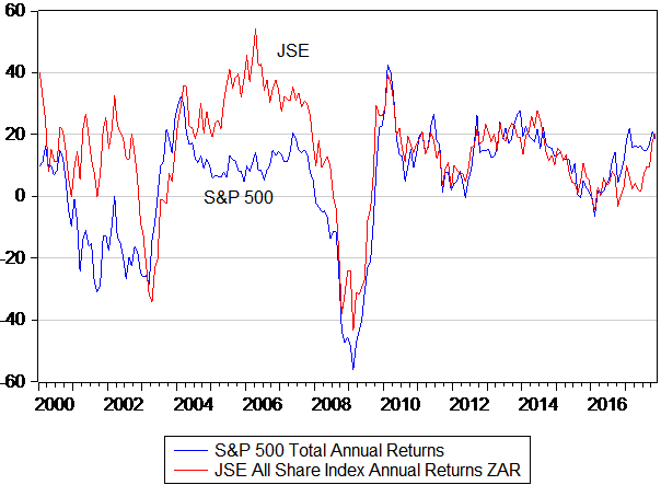
Source: Iress and Investec Wealth & Investment

These total share market returns (price changes and dividends received) have been calculated as gains or losses realised over the previous 12 months and calculated each month. The average annual return on the S&P 500 between January 2000 and November 2017, in US dollars, was 5.3% compared to 14.4% in rands generated on the JSE. The worst month for both markets was in late 2008, when both markets were down over 50% on the year before. The best year-on-year return on the S&P 500 over this period was 43%, realised in the 12 months to February 2010, while the best months for investors on the JSE were in late 2005 when annual returns peaked at over 50%. Adjusted for inflation in the US and SA, the S&P Index has provided about a real average 3% p.a return and the JSE an impressive 8% p.a. in real rands.

When measured in US dollars, the JSE also outperformed, having delivered close to 7.5 % p.a on average compared to the 5.3% p.a earned on the S&P 500. It may be seen in figure 2 below that the JSE provided superior US dollar returns between 2003 and 2007, but offered markedly inferior returns (in US dollars) compared to the S&P 500 since 2012. These high average returns over an extended period of time surely indicate the advantage of maintaining consistently high exposure to equities over the long run.

Figure 2: annual US dollar returns – S&P 500 Index and the JSE All Share Index

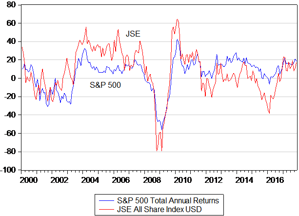
Source: Iress and Investec Wealth & Investment

While timing which market to favour over another – the JSE before 2008 and the S&P 500 after 2014 – can make an important difference to investment outcomes, it should also be noted that the returns on the S&P 500 and the JSE are quite highly correlated on average (close to 70%) in all the ways to measure performance.

The forces common to all equity markets around the world will often be directed from the US economy and its asset markets to the rest of the world – rather than the other way round – making an analysis of the state of the S&P 500 a very good starting point for analysing any equity market.

The essential question then arises. Is it possible to undertake value-adding or loss-avoiding equity market timing decisions with any degree of analytical conviction? Such market timing decisions are unavoidable for any fund manager or investment strategist with responsibilities for funds that are not all-equity funds. Any fund required by its investors to hold a balance in their portfolios of cash, fixed interest investments of various kinds as well as the many alternative asset classes that might feature in portfolios, would have to exercise judgements about the risk inherent in equity markets at any point in time.

The risk that the equity markets might, as they have in the past, melt down or even melt up – only then perhaps to melt down again – must therefore be uppermost in the minds of all fund managers having to decide on an appropriate allocation of assets. Even those running all equity funds have to decide how to time turning newly entrusted cash into equities and, more important still, which particular equities to buy and sell.

The broad direction of the equity or any other market can only be known after the event. From day to day, month to month or quarter to quarter, market prices and values are about as likely to go up as they are to go down. These short-term price moves therefore appear to observers as largely random, as the figure of monthly changes and daily moves in the S&P 500 Index shown below demonstrate. Note the still random (down/up, up/ down in no predictable order or magnitude) but very wide daily moves in the S&P 500 during 2008-2009 and during the euro bond crisis of 2011.

Figure 3: S&P 500 monthly returns (percent)

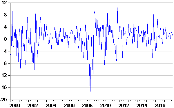
Source: Iress and Investec Wealth & Investment

Figure 4: S&P 500 daily returns (2005-2017)

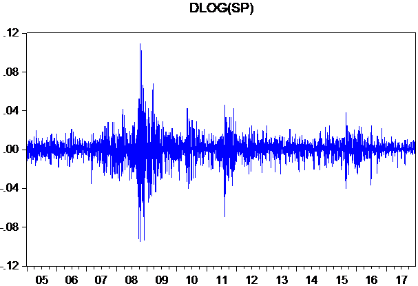
Source: Iress and Investec Wealth & Investment

But these daily or monthly movements may reveal a broad drift in either direction, more up than down, or the other way round, measured over longer period of time. So when daily and monthly moves are converted into annual changes, observers will get the drift (after the event) and a persistent statistically smoothed trend in returns, that peaks and troughs in some more regular way, will be registered, as shown in figures one and two above. These phases, from top to bottom in annual returns, are defined as either a bull or bear market or something in between, depending on the depth or height of the following trough or peak, but can only be identified with hindsight.

Understanding how assets are valued

This does not mean that nothing meaningful can ever be said about the state of a market after it has moved higher or lower. With observation of the past we can understand the forces that have driven the value of any company higher or lower and so the average of them represented by a stock market index and therefore recognise the forces that might drive them higher or lower in the future, if past performance can be relied upon.

Successful, more profitable companies – those that earn a high return on the capital shareholders provide their managers – after all command higher values than less successful ones. And part of their success or failure will also have to do with the environment in which they operate. The laws and regulations, including the taxes their shareholders are subject to, will influence their ability to generate revenues and reduce costs, as will fiscal and monetary policies. The more certainty about these forces in the future, the less (more) risk to be discounted in the prices paid and the more (less) valuable will be the future flows of revenues and costs in which owners will share.

These market wide forces that determine the value of a share market index are in principle not difficult to identify. In practice they raise many unresolved issues about how best to give effect to the underlying theory. The economic caravan always moves on making it impossible to prove the superiority of one valuation approach over another. Holding other things equal is only possible in the laboratory, not in the economy.

The market can be thought of as conducting a continuous net present value (NPV) calculation, estimating a flow of benefits from share ownership over time, the numerator of the equation. That can be calculated as earnings (profits) or dividends or net (free after-capital expenditure) cash flow expected. The calculations of these are highly correlated when measured for an aggregate of all the firms that make up the Index. This expected performance of the market is then assumed to be discounted by a rate that reflects the required risk-adjusted rate of return set by the market.

The cost of owning shares rather than other assets, is given effect in the applied discount rate. It represents the opportunity foregone to own other assets, for example government or private bonds or cash, that offer pre-determined interest rate rewards with less default risk. In addition shareholders will, it is assumed, expect some additional reward, described as an equity risk premium (ERP) for the extra risks incurred in share ownership that offer no predetermined income. Hence a higher discount rate when the ERP is added to benchmark, default risk free fixed interest rates as provided by securities issued by a government. Such risks can be measured by the variability of the value of the share index from day to day, as shown above, a process of price determination that makes share prices more variable and less predictable than those of almost all other relevant asset classes.

These share prices will go up or down as the discount rate rises or falls with changes in interest rates. And with circumstances that cause investors to attach more uncertainty to the flow of benefits they expect from share ownership. The price of the shares goes lower or higher to compensate for these extra or reduced risks to the outlook for the economy and the companies who contribute to it.

The numerator of the NPV equation that summarises the expected flow of benefits to owners may be regarded (for reasons of simplicity) as (relatively) stable. A lower (higher) share price reconciles this given outlook with the required risk adjusted return that makes owning a share seem worthwhile. So when discount rates go up (down) – valuations (share prices) move in the opposite direction to improve (reduce) the expected returns from share ownership. Lower prices, other things being equal including expectations of profits to come, mean higher expected returns and vice versa.

Understanding and taking issue with the market consensus

One of the essential questions with which to interrogate the market, is to judge whether current market-determined interest rates are likely to move higher or lower or the environment that companies will operate in is going to become more or less helpful to their profitability. By definition, what surprises the market moves in interest rates or tax rates or risk premiums, will move valuations in the opposite direction. You may believe that the marketplace has misread the true state of affairs, such as the outlook for interest rates and risk premiums, and so has mispriced the share market, overvaluing or undervaluing it enough to encourage additional selling or buying.

The market consensus (revealed by the current level of the Index) will also have incorporated its expectations of performance to come by the companies represented in the Index. This consensus may also prove fallible. Earnings may be about to accelerate or decelerate in surprising ways. Operating profit margins may stay higher or lower for longer than expected. The economy itself may be about to enter an extended period of well-above past growth rates. If so, and you will have your own reasons for believing so, this would provide good reason to reduce or increase exposure.

Such contrarian opinions, if acted upon will add to or reduce exposure to equities. The market consensus is determined by its participants, all with the same incentive to understand it better, as you have, and is studied by many with great analytical skills and vast experience. Consensus has every reason to be the consensus. And when the consensus changes – as we have shown it so often changes – it will do so for good and well-informed reasons. Beating the market – that is getting market timing right – is a formidable task, so humility is advised.

While perfectly timing market entry or exit is not a task given to ordinary mortals, we can draw some helpful inferences about the condition of the market place, given this sense of what has driven past performance. We are in a position to judge how appropriately valued a market is at a point in time and therefore what would be required of the wider economic forces at work to take the market higher- or prevent it from going lower. We will attempt to recognise what is being assumed of the equity market – what assumptions are reflected in the prices paid for shares – and whether or not you can agree or differ from what is at all times the market consensus.

Our valuation exercises

We judge whether the equity market is demandingly or un-demandingly valued in the following way. We determine how current valuations are more or less demanding of additional dividends. Why dividends? Because they have the same meaning today as always: cash paid out to shareholders rather than retained by the enterprise. They are not subject to changing accounting conventions, such as the nature of capital expenditure and research and development expenditure that may or may not be fully expensed to reduce earnings. What may appear as an overvalued market would need a strong flow of dividends to justify current values and expectations. An undervalued market would be pricing in a slow-down in dividend payments. Good or poor dividend flows can take the market higher or lower.

Furthermore, we judge whether the market is more or less complacent about the discount rates that will be attached to these dividends to come. In this we are also aware that the interest rates we observe and that the market expects, as revealed by the level of long term interest rates and the slope of the yield curve, may be abnormally low or high – but might normalise to some degree in the near future.

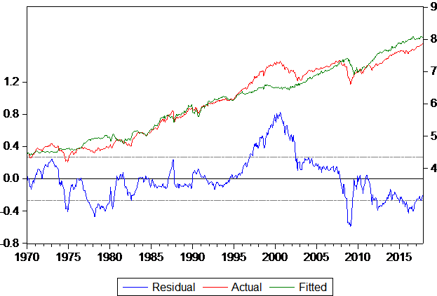
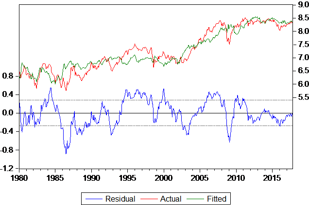
We utilise regression equations that compare the current level of the leading equity index the S&P 500 to the level predicted by trailing dividends and long-term interest rates. The results of such an exercise are shown below. The model equation predicts a significantly higher S&P 500 than is the case today, some 40% higher. By this standard the S&P is currently undervalued.

The model provides a very good fit and both explanatory variables easily pass the test for statistical significance and accord well with economic theory. It explains past market behaviour well.

Figure 5: Regression model* of the S&P 500 (1970-2017)

Source: Iress and Investec Wealth & Investment

*Representation:

LOG(SP) = -1.80463655704 + 1.18059721064*LOG(SPDIV) – 0.0727779346562*USGB10

We can back test the model. If the model was run with data only up to November 2014 when the S&P began its new upward momentum we would have received a very helpful signal that the S&P was in fact very undervalued at that time. This signal would have encouraged investors at that point in time to have maintained high equity weight in portfolios- or what is described as a risk-on position.

Similarly had we applied the model in early 2000, just before the so called Dot.com bubble burst, the model would have registered that the S&P 500 Index was then greatly overvalued for prevailing dividend flows and interest rates Reducing exposure to equities at that point in time would have been very much the right approach to have taken – as we soon came to find out. We should add however that the model would also have registered a high degree of overvaluation as many as three years before the market fell away from its high peak. Even irrational exuberance, as Alan Greenspan memorably described it in 1997, perhaps relying on a similar approach to value determination, or its reverse undue pessimism, can persist for an extended period of time, making our model or any such valuation exercise based on historical performance unhelpful as a short-term trading model, but still valuable as a basis with which to interrogate market consensus.

In our models we regard the value of the S&P 500 as representing the present value of a flow of dividends (the performance measure) discounted by its opportunity cost, represented by the interest rate (the expected return) on offer from a 10-year US bond yield. An alternative approach would be to compare the value of the Index to the expected economic performance of the companies included in the Index, and then to infer the discount rate that could equalise price and expected performance in the NPV equation.

The Holt system[1] undertakes this calculation. It estimates the free cash flow return on capital realised by and expected from all listed companies (CFROI) real cash flow return on real cash invested using the same algorithms applied to all the companies covered by the system and its data base. This analysis can be used to derive a market discount rate for any Index that equalises the value of an Index, for example the S&P 500, to the cash flows expected from it.

In the figure below we compare this nominal Holt discount rate for the S&P 500 to US long term interest rates. These discount rates have receded with long-term interest rates, as theory would predict. Note also that both interest and the Holt discount rate are at very low levels, implying higher share prices for any given flow of dividends.

Of greater importance perhaps for share prices than discount and interest rates is the spread between them. This spread, the extra risk premium for holding equities rather than bonds, has widened in recent years. While the discount rate may have declined, it has maintained and even increased the distance between it and interest rates, so encouraging demand for equities.

When we replace interest rates with this risk premium in our dividend discount model we get a very similar signal of a currently undervalued S&P 500 (see below).[2]

Figure 6: US Holt discount rates (nominal) US long bond yields (10 year) and risk spread

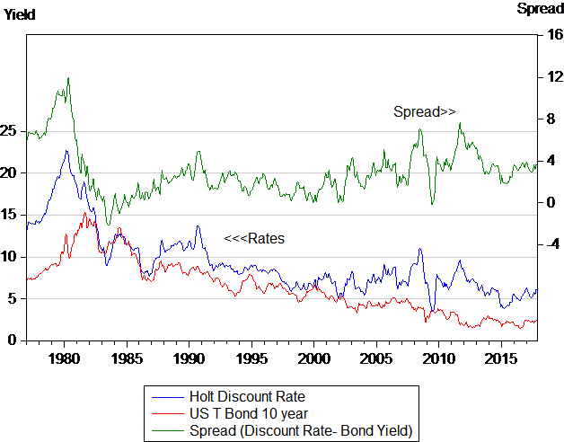
Source: Credit Suisse Holt, Iress and Investec Wealth & Investment

Figure 7: Real Holt discount rates and real interest rates and real risk spread

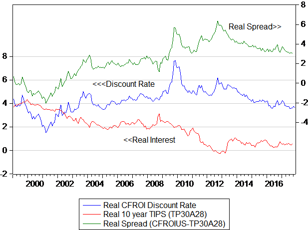
Source: Credit Suisse Holt, Iress and Investec Wealth & Investment

Figure 8: A model of the S&P 500 (explanatory variables, dividends and spread between discount rate and long term interest rates)*

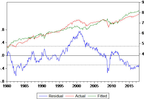
*Representation of the equation:

LOG(SP) = -4.59846533561 + 1.51940769795*LOG(SPDIV) – 0.0501430590849*(CFROINOM-USGB10)

Source: Credit Suisse Holt, Iress and Investec Wealth & Investment

Therefore we conclude that the S&P 500, despite its recent strong upward momentum, is undervalued for current dividends and interest rates or the risk spread. However some caution about the level of the S&P Index is called for by a sense that long-term interest rates are now very low and may well normalise. A further reason to be cautious about the current level of the S&P 500 is that the day-to-day volatility of the Index has been very low by comparison with the past. This indicates an unusual degree of comfort with the current state of the US share market. Were volatility to normalise, share prices would probably under pressure.

Hence our asset allocation advice has been to retain a neutral exposure to equities for now, with the next 18 months in mind. On a shorter term view (less than six months) however, we are of the view that upside strength is at least as likely as any move lower.

When we review the JSE applying a similar method of analysis, the rand values of the All Share Index appears as fairly valued for trailing dividends and US Interest rates. It also appears fairly valued when all the variables of the model are converted into US dollars. However when the (high) level of the S&P is included as an explanation of the USD value of the JSE in place of US interest rates the JSE appears as now attractively undervalued.

The S&P 500 is normally a rising tide that lifts all boats. But in the case of the JSE this has not been the recent case. Not only the JSE but emerging market equity indexes generally also lagged behind the S&P 500 after 2014 and until mid-2016. It will take less SA risk, which comes with an improved political dispensation, to focus global attention on the potential value in SA equities, particularly the companies heavily exposed to the SA economy. The SA political news has improved and the case for SA equities exposed to a potentially stronger SA economy, has also improved, making the case for a somewhat overweight exposure to this sector of the JSE.

Figure 9: A model of the US dollar value of the JSE with dividends and US interest rates*

*Representation:

LOG(JSE USD ) = 1.3925529347 + 0.776827626347*LOG(DIVIDENDS USD ) – 0.127168505553*US 10 Y Bond Yields

Source: Credit Suisse Holt, Iress and Investec Wealth & Investment

[1] Credit-suisse.com/holtmethodolgy

“HOLT derives a market-implied discount rate by equating firm enterprise value to the net present value of free cash flow (FCFF). HOLTs FCFF is generated by a systematic process based on consensus earnings estimates, a growth forecast, and Fade. This process is similar to calculating a yield-to-maturity on a bond” See Holt Notes November 2012

[2] In order to undertake the analysis over an extended period of time we added US inflation to the real Holt discount rate for the US sample to establish a nominal discount rate to be compared with nominal interest rate. An equivalent series of US real interest rates (Tips) is only available from 1997

The great taskmaster

The success of any business enterprise is measured by the return realised on the capital entrusted to it. The managers of an enterprise will rationally direct the capital provided them to particular business purposes in the expectation of a return on the capital invested that exceeds its opportunity cost, that is greater than the expected return from the next best alternative project with similar risks of success or failure. The more risk of failure, the greater must be the required (breakeven) return.

Measuring the internal rates of return delivered by an operating enterprise in a consistent way over any short period of time, for example a year or six months, has its own accounting for performance complications. The fullness of time, or until the venture is sold or liquidated, may be necessary for calculating how well the owners have done with their capital. However calculating the risks of failure of any potential project is much more a matter of judgement and sound process, than any precise measurement.

The only returns that can be measured with accuracy are those realised for investors in listed and well-traded companies. Returns come explicitly in the form of capital gains or losses and dividends or capital repayments received. And risks to potential returns are measured by the variability of these (monthly) returns over time that hopefully have a consistent enough pattern. A consistency furthermore that identifies the returns from a company as more or less risky compared to the pattern of average returns realized on the stock market. These measures can then form the basis of a required risk-adjusted return for a company or an investor to aim at.

These so-called betas that compare returns on individual shares to market returns as above or below averagely risky may in fact be quite unstable variables when measured over different time periods. Furthermore, these equations that relate company returns to market returns may or may not explain a great deal of past realised returns. The alpha of the total return equation that reveals company specific influences on total returns may account for much of realised returns.

This may be as well when judging the competence of the managers deciding and executing on projects. If the share market returns are mostly alpha (under the control of manager) and not the result of market wide developments over which managers have no influence, then determining the contribution of managers to realised returns becomes a consistent process.

Those buying a share from a willing seller are mostly gaining a share in the established assets and liabilities of an operating company – a share that the seller is willingly giving up – at a price that satisfies both. They are not providing extra capital for the firm to employ.

By establishing a price for a share they are however providing information about the market value of the company’s operations and so by implication the terms on which the company could raise further share or debt capital, should they wish to do so to supplement the company’s own savings to be invested in ongoing projects. The additional capital invested by operating companies will mostly be funded through cash retained by the firm, that is from additional savings provided by established shareholders.

The secondary share market transactions, through their influence on share prices, converts the internal rates of return realised by and expected of an operating company, into expected market returns. The superior the expected performance of an operating company, the more investors will pay up in advance for a claim on the company. The higher (lower) the share price the lower (higher) must be the expected returns for any given operating outcomes.

In this way through share price action, higher costs of entry into the investment opportunity, companies and their managers that are expected to generate way above average returns on the capital they invest in on-going operations and projects, may in reality only provide market-related average returns to share owners over any reporting period, say the next year or two. The further implication of these market expectations, incorporated into share prices, is that only a surprisingly good or disappointing operating results will move the market. The expected will already be reflected be in the price of a share or loan.

The implications of these expectations and their influence on share market prices and share market returns for managers and their rewards, provided by shareholders, seems obvious. Managers should be rewarded for their ability to realise or exceed the required internally generated returns on capital invested: charged to exceed targets for internal rates of return that are set presumably and consistently by a board of directors, acting in the interest of their shareholders.

Better still, targets set for managers that are made public and well understood and can be defended when exceeded and managers who are then rewarded accordingly. By contrast, share market returns that anticipate good or poor performance, cannot reveal how well or poorly operating managers have done with capital entrusted to them. Rewarding operating managers on the basis of how their shares performed is not a good method. Excellent companies that are expected to maintain their excellence and perform as expected to very high standards may only generate average returns. And poor management can wrongly benefit from above normal returns if expectations and share prices are set low enough. The correct basis for recording the value of managers to their shareholders is to recognise as accurately as possible, the realised internal rates of return on the shareholders capital they have employed.

The managers of companies or agencies that invest in operating companies – be they investment holding companies or unit trusts or pension funds – can however be judged by the changing value of the share market and other opportunities they invest in. Their task is to earn share market beating risk adjusted returns. They can only hope to do so by accurately anticipating actual market developments. They can do so anticipating the surprises that will move the market one way or another and allocating capital accordingly in advance of them.

The managers of a listed investment holding company, for example a Remgro or PSG or a Naspers, are endowed with permanent capital by original shareholders that cannot be recalled. This allows them to invest capital in operating companies for the long run. They, the managers of the holding company, when allocating capital to one or other purpose, must expect that the managers of these operating companies they invest in are capable of realising above average (internal) returns on the capital they invest. If indeed this proves so, they must hope that the share market comes to share this optimism and prices the holding company shares accordingly, to reflect the increased value of the assets it owns. Other things being equal, the greater the market value of their investments the greater will be the market value of the holding company.

But other things may nor remain the same. The market place is always a hard task master. Past performance, even good investment management performance, may only be a partial guide to expected performance. The capabilities of the holding companies’ managers to add value by the additional investment decisions they are expected to make today and tomorrow – not only the investments they made in the past – will also be reflected in the value attached to their shares.

These can stand at a discount or at a premium to the market value of the assets they own. The difference between the usually lesser market value of the holding company and the liquidation value of its sum of parts – its NAV – will reflect this pessimism about the expected value of their future investment decisions.

A lower share price paid for holding company shares compensates for this expected failure to beat the market in the future – so improving expected share market returns. It is a market reproach that the managers of holding companies should always attempt to overcome, by making better investment decisions. And by exercising better management of their portfolios, including converting unlisted assets into potentially more valuable listed assets and also by indicating a willingness to unbundle successful listed assets to shareholders when these investments have matured. And be rewarded appropriately when they succeed in doing so.

21 December 2017

The SA economy – some Christmas cheer

The incipient cyclical recovery identified in our last report on the state of the SA economy has been confirmed by the most recent data releases. New vehicle sales and the supply of cash to the economy at November month end both support the view that the economy is demonstrating resilience.

We combine these up to date, hard numbers (not based on sample surveys) to calculate our Hard Number Indicator (HNI) of the business cycle. As we show in figure 1 the HNI is now pointing higher after showing little momentum after 2014 and having moved lower in 2016. The annual change in this indicator (the second derivative of the business cycle) has moved into positive territory and is forecast to maintain this momentum.

The components of the HNI are shown below. The real money base, the note issue, adjusted for the CPI (to November 2017) has become less negative while the new vehicle sales have maintained an encouraging revival.

If recent vehicle sales trends are maintained, new vehicle sales would be running at a 600 000 unit rate at year end 2018. This would represent a welcome recovery from the cyclical trough of mid-2016 but would still leave sales well below the previous peak rates of 2006 and 2012-2014.

Sales volumes at retail level, excluding motor vehicles, have been reported for October 2017. They show that the retail sales cycle continues its upward momentum and is pointing to growth rates of about 3% through 2018. This growth will be assisted by the growth in demands for cash. Extra cash is still a very good coinciding indicator of retail spending intentions despite all the digital alternatives to cash in SA (see figure 4).

Perhaps a more important encouragement for households to spend more is that prices at retail level have hardly increased over the past few months. The retail price deflator has moved sideways even as the CPI continues its upward trend, though also at a more modest rate. Hence the trend in inflation at retail level is sharply lower and, if sustained, will prove a stimulus to spending (see figures 5 and 6). The key to the door of lower prices at retail level is the exchange value of the rand. The outcome of the ANC succession struggle at Nasrec this weekend will be well reflected in the rand and in turn in retail spending and inflation. 14 December 2017

ANC elective conference – what are the odds?

The markets have been recording their judgements about the outcome of the battle to succeed President Jacob Zuma as leader of the ANC to be decided over the next few days. The prospects of Cyril Ramaphosa succeeding has been recorded in the degree of rand strength versus its emerging market peers. As we show in figure 1 below, the rand weakened in response to the appointment of Minister of Finance Malusi Gigaba in March and weakened further after he presented his mini-Budget statement in October. Since then, and despite a very critical report from the credit rating agencies and a downgrade, the rand has recovered strongly – in an important relative sense – and not only versus the US dollar.

The same improvement in sentiment is revealed in the market for US dollar-denominated RSA bonds. As we show in figure 2, the spread between the interest rate yield on five-year RSA bonds and five-year US Treasury bonds that offers compensation for extra SA risks of default, has also narrowed from 2.2% in early November to about 1.8% on 14 December.

A still more direct measure of the probabilities of one or other candidate being first past the post is provided by online sportsbook operator Sportingbet (https://www.sportingbet.co.za).

When their books first opened the odds on the various potential candidates – or those not yet identified were as shown below. The favourite was Nkosazana Dlamini-Zuma with a 42% chance of winning (1/2.4) while Cyril Ramaphosa was given only a 27% probability of winning, less than the chances of Zweli Mkhize.

The decimal odds are now as shown below. Ramaphosa is the firm favourite, given a 57% chance of winning compared to a 33% chance for his closest rival Dlamini-Zuma. The odds on any other outcome have blown out.

The volume or value of bets cast is not disclosed, but we are informed by Sportingbet that 65% of the bets and 61% of the stakes have been cast for Ramaphosa, while 21% of the bets have been placed on Dlamini-Zuma and a larger proportion (36%) of the stakes cast for her. These books will close on Saturday 16 December and we are informed by the firm, who describe themselves as operator of South Africa’s largest online sportsbook:

“Unfortunately, as part of our trading risk management policy, and as a company policy, we never disclose amounts wagered, numbers of bets, or users on any single event. I can share however that considering it’s a “novelty” (or non-sporting event) market, the bet activity and interest on this is impressive. “

There is a great deal at stake for the economy in the ANC race for the top. Clearly, judged by the markets and the odds and the politically savvy involved, there are no certain outcomes. Were therefore the favourite to win and the more decisive the victory, the stronger the rand and the lower the risk spreads – and so the chances of a strong SA economic recovery. Perhaps something those casting their votes might bear in mind. 15 December 2017

Hail to the SA consumer

The South African economy cannot be said to be performing to its potential. But in one important sense it is performing well – for consumers. Those with income or borrowing capacity will not find the economy wanting when they come to exercise their spending choices over the holiday season.

The shops will be well stocked and able to meet their every demands and desires, be it for essentials or luxuries supplied from all parts of the world. They will not lack for bread or toilet paper or for wine, beer or spirits. Or lack for wonderful world class entertainment at the theatres and movie houses. The book shops will be well stocked for those who still regard reading as entertaining and valuable. Excellent restaurants of all ethnic persuasions will be open to them, but may require an advance booking, given the competition from foreign tourists, who are showing their increased appetite for what we enjoy at the prices we pay.

This is as it should be. Successful economies gained their cornucopias by putting the demands of consumers in first place. That is preventing producers, farmers or factory owners or avaricious rulers or ecclesiastical orders or soldiers to decide what is to be produced. And when consumers largely rule the economy and producers are required to respond to them, economies flourish. Doing it the other way round – for the state to put the interest of producers, including those employed by them – whose own well-being is always threatened by competition – is a recipe for economic failure and for stagnation and corruption and the waste of the opportunity to consume more.

A consumer-led economy need ask very little of the state. The State and its officials will not be called upon to design industrial policy or determine development plans, policies that require foresight that is simply not available to even the best informed and least self-interested official. What the effective State has to provide is the protection of contracts freely entered into and the capital of those who have saved and puts their capital and skills to work, hoping to satisfy their customers and be rewarded for doing so.

The state should also ensure that the success or failure of businesses, large and small, is determined by their sales to customers and the costs of doing so. Not where financial success is dependent on an ability to negotiate a morass of regulation and relations with powerful officials. This system inevitably advantages bigger business over their smaller rivals.

A consumer-led economy is a continuous process or trial and error, of firms learning and adapting to unpredictable circumstances. The winners and losers for the consumers’ spending power emerge – they are not chosen by planners. South Africa incidentally, since 1994, has spent hundreds of billions of rands – perhaps over 400 billion rands of them – in subsidising industries of one kind or another with taxpayers’ money or tax concessions, money that could have been put to much better effect by consumers, especially poor ones.

The South African government alas appears only too willing to continue to put producers and officials first. For example competition policy is directed to serve industrial and labour policy rather than protect consumers.

More important for economic development, given that education and training precedes the ability to produce, earn and consume more, it is tragically the educators, the producers, who are first in line when the huge government budgets for such purposes are allocated. Were the taxpayer to pay the fees to enable all those desperately seeking education and training to attend private schools, universities and training establishments, of their own choosing, the valuable customer would come first. And the outcomes in the form of additional employment and incomes would be far superior.

The market for jobs in South Africa – why it performs so poorly and what can be done to improve it

Piece written for the Free Market Foundation: http://www.freemarketfoundation.com/publications-view/the-market-for-jobs-in-south-africa-%e2%80%93-why-it-performs-so-poorly-and-what-can-be-done-to-improve-it-

A pdf version is also available here.

Exchange rate risks for international businesses and investors: why South Africa is not unique

The global economy remains hostage to a volatile US dollar

The US dollar continues to serve as the primary international unit of account and as the pre-eminent reserve currency held by central and other banks, yet the rate at which the US dollar is exchanged for other currencies remains vulnerable to large moves in both directions, so adding risks to all financial transactions that make reference to it. In figure 1 below, we show the performance of the US dollar against its developed market peers (The US dollar index or DXY). We also show the real dollar exchange rate against the same major trading partners. The real exchange rate adjusts the nominal trade-weighted exchange rate for differences in inflation rates. We discuss the economic importance of real exchange rates further below. However, it should be noted that the real and nominal US exchange rates have followed a similar pattern.

Figure 1: The trade-weighted real and nominal exchange value of the US dollar (1975=100)

Sources: Bloomberg, The Federal Reserve Bank of St. Louis (Fred Data Base) and Investec Wealth & Investment

In figure 2, we show the performance of the US dollar against its developed market peers, an index of emerging market exchange rates since 2010 that excludes the rand, and the rand/US dollar rate.

Figure 2: The US dollar vs. major currencies, an emerging market currency basket and the rand (higher numbers indicate exchange rate strength), monthly data (2010=100)

Sources: Bloomberg, The Federal Reserve Bank of St. Louis (FRED database) and Investec Wealth & Investment

The extraordinary strength of the US dollar in 2014 was associated with a high degree of emerging market (and rand) exchange rate weakness. Also note that a degree of US dollar weakness that begins in mid-2016 has been associated with a recovery in the emerging market basket (and the rand). US dollar volatility poses particular challenges for monetary policy in emerging economies. We return to this important issue below.

The real exchange rate is what matters for real business activity

Inflation can make a producer or distributor of goods or services less competitive in home and foreign markets. However, a weaker exchange rate can protect operating margins against those rivals subject to less inflation. What may be gained or lost in the ability to compete on price – when expressed in any common currency – can be offset by changes in the rate of exchange.

When the offset is complete, the exchange rate will have weakened or strengthened by the percentage differences in inflation in the home country and that of its trading partners. If such circumstances, the exchange rate would be said to conform to purchasing power parity (PPP). Thus, PPP is regarded as a theoretical equilibrium to which exchange rates will converge in time.

The deviations from PPP-equivalent exchange rates are used to calculate a real exchange rate. It is this real exchange rate that defines the competitiveness of prevailing market-determined exchange rates. A real exchange rate with a value of more than 100 indicates an overvalued exchange rate and a value less than 100 indicates a competitive or undervalued exchange rate. The direction of the real exchange rate towards or away from 100 shows whether domestic producers have become more or less internationally competitive.

The calculation of a real exchange rate can include multiple exchange rates and an equivalent number of inflation rates – weighted by the share of imports and export held by different trading partners. The prices of relevance for the calculation of inflation and the real exchange rate are usually derived from prices charged for the manufactured goods that are presumed to dominate international trade.

The history of flexible exchange rates in SA shows that, the USD/ZAR exchange rate as well as the trade-weighted rand exchange rate, have consistently deviated from PPP-equivalent exchange rates and in varying degrees (see figures 3 to 5). This indicates that when SA firms engage in foreign trade and have to compete on the domestic market with imports this is a risky activity, given the variability of the real exchange rate and operating margins.

Measuring real exchange rates – a focus on South Africa

These divergences from PPP-equivalent exchange rates, i.e. fluctuations in the real rand exchange rate, are large and variable. This real rand exchange rate volatility for the rand is linked to the removal of exchange controls on foreign investors that were effectively withdrawn in 1995. There was a brief period of real exchange rate volatility, between 1983 and 1985, when foreign investors were also free to move funds into and out of South Africa. A further source of capital flows has been the progressive relief on the exchange controls applied to South African residents.

Freer capital flows rather than trade flows have dominated the demand for and supply of rands exchanged for US dollars and other currencies, and has introduced significantly more rand exchange rate volatility . It is the flow of global capital that has similarly dominated exchange rate trends in all economies that are open to this free flow of capital.

As we show below, using January 1970 as the starting point, the USD/ZAR exchange rate diverged significantly from PPP in 1985, then conformed to PPP between 1988 and 1995, whereafter the divergence has been continuous, though still highly variable. Heavy shocks to the USD/ZAR exchange rate are to be observed in 2001-02, 2008 and 2014. These sharp deviations from PPP have been followed by movement back towards PPP.

Sensitivity to the base year

Notice too that the PPP calculation is sensitive to the base year used to calculate the price indices. When 2010 is taken as the starting point for the calculation, the absolute deviations from PPP exchange rates are of a different magnitude. However, the movement away from or back towards PPP-equivalent exchange rates takes the same direction in both versions of PPP-equivalent exchange rates.

The starting point for any such calculation should be when the actual exchange rate approximates PPP, as it did in 1970. By 2010, the base year for calculating the current real exchange rate, the USD/ZAR exchange rate had moved far away from PPP, using a 1970 base year. When the base year is taken to be 2010, the rand appears as less undervalued generally and even as overvalued in 2010 – when the USD/ZAR traded at less than its PPP equivalent (2010 prices).

Figure 3: Market and Purchasing Power Parity exchange rates (USD/ZAR) (1970=100)

Sources: Stats SA, Federal Reserve Bank of St. Louis (FRED Data Base), Investec Wealth & Investment

Figure 4: Market and Purchasing Power Parity exchange rates (USD/ZAR) (2010=100)

Sources: Stats SA, Federal Reserve Bank of St. Louis (FRED database) and Investec Wealth & Investment

In figure 5 below we show the ratio of the PPP-equivalent USD/ZAR exchange rates to the market-determined USD/ZAR, using 1970 or 2010 as the base year. This ratio may be regarded as representing the real USD/ZAR exchange rates. Values above 100 indicate an overvalued (less competitive) nominal exchange rate and values below 100 indicate the opposite – the nominal exchange rate has changed by more than the difference in inflation in SA and the US.

Using 2010 prices and exchange rates, the rand was overvalued for much of the period from 1970 to 1995 and for some years afterwards. The strong real rand was supported in the 1970s by rising gold and metal prices in US dollars. The picture using 1970 prices as the basis of the calculation is different, revealing a consistently undervalued rand after 1985.

Figure 5: USD/ZAR – the ratio of PPP to market exchange rates; a measure of the real exchange rate using different base years

Sources: Stats SA, Federal Reserve Bank of St. Louis (FRED database) and Investec Wealth & Investment

Real exchange rates considered more widely – the international evidence

In the figures below, we show a variety of trade-weighted real exchange rates for the period 1995-2017, as calculated by the Bank for International Settlements and the SA Reserve Bank. All these real exchange rates are highly variable, including those of the US. The real US dollar demonstrated continuous strength between 1995 and 2002, then weakness to 2008, whereafter the safe haven status of the US dollar in a time of crisis added some real strength to the trade-weighted exchange rate. A further period of pronounced real dollar strength ensued after 2014. Not coincidentally, the real trade weighted rand moved in very much the opposite direction, as seen in figure 6.

It should be recognised that the real rand, for all its volatility and the risks to which it has exposed SA business, has not in fact been more variable than the real dollar. As a relatively small economy that is very open to foreign trade, real exchange rates are, of course, more important for the South African economy. The value of exports and imports for South Africa is equivalent to about 50% of GDP. The exposure to imports and exports in the US is equivalent to about 30% of GDP.

As may be seen in the figures below, the real euro and real sterling have also been highly variable since 1995, while the Brazilian real has been more variable than most. The summary statistics for these real exchange rates are provided in Table 1.

The conclusion, therefore, is that the volatility of the real rand that so complicates the business of exporting from and importing to SA is not exceptional. The same complications and risks of doing business across frontiers, or rather exchange rate regimes, apply across the modern world of flexible exchange rates. It should be recognised that flexible exchange rates have added generally to the risks of doing international business everywhere. As such, these risks are presumed to have increased the required returns on capital invested in servicing global markets.

One can also determine whether there is a general tendency of exchange rates to revert to PPP and foreign trade-neutral real exchange rates. In other words, can one conduct a statistical test of whether real exchange rates are mean reverting?

The answer is that they don’t pass this statistical test with any degree of statistical confidence. The Chinese and Japanese real exchange rate trends since 1995 are most conspicuously not mean reverting to the theoretical 100 as may be observed in figure 9. The real yuan has a distinct and persistently stronger trend while the real yen moves persistently weaker.

Figure 6: Real exchange rates 1995-2017, South Africa and the US (2010=100)

Source: SA Reserve Bank, Federal Reserve Bank of St. Louis (FRED database) and Investec Wealth & Investment

Figure 7: Real exchange rates 1995-2017, South Africa and Brazil (2010=100)

Source: SA Reserve Bank, Federal Reserve Bank of St. Louis (FRED database) and Investec Wealth & Investment

Figure 8: Real exchange rates 1995-2017, UK and Eurozone (2010=100)

Source: SA Reserve Bank, Federal Reserve Bank of St. Louis (FRED database) and Investec Wealth & Investment

Figure 9: Real exchange rates 1995-2017, China and Japan (2010=100)

Source: SA Reserve Bank, Federal Reserve Bank of St. Louis (FRED database)and Investec Wealth & Investment

Table 1: Real exchange rates summary statistics

The importance of capital rather than trade flows in determining nominal and real exchange rates

The notion that exchange rates will trend, over time, back towards some kind of competitive equilibrium, as imports and export volumes adjust to the real exchange rate effects on operating margins, therefore does not hold. The volatile behaviour of both nominal and real exchange rates is driven by unpredictable capital flows rather than by flows of currencies generated by the international trade in goods and services.

These capital flows that are based upon changing expectations of future returns, move the rate of exchange stronger or weaker. Inflation rates then react, but not rapidly or sufficiently enough to sustain PPP.

The exchange rate therefore leads inflation and the nominal exchange rate leads the real exchange rate – because inflation rates are much more stable than exchange rates. This stability is partly the result of the convention that measures inflation as the year-on-year change in consumer or other price indices, rather than as price moves over shorter periods of time. For example, a one or three month trend in consumer prices would indicate much more variability. The variability of real exchange rates has, in practice, almost everything to do with shocks to nominal exchange rates rather than price.

The shocks to the real exchange rate observed in the charts above therefore have very little to do with shocks to inflation rates. The openness of an economy to imports of staple commodities reduces the impact of harvests that are subject to unfavourable climatic conditions. Droughts and famines might otherwise have pushed prices temporarily much higher, providing a price shock to the economy.

As we show in figure 10 below, annual moves in the nominal ZAR/USD exchange rate dominate the moves in the real rand exchange rate that are so important for operating businesses and their operating profit margins. Similar results could be found for many other economies and their currencies as was found to be true of the US demonstrated in Figure 1

Figure 10: Annual changes in the USD/ZAR nominal and real exchange rates

The impact of exchange rates on prices and inflation

Exchange rate shocks will have implications for the domestic price level. Other things being equal, the price of imported goods and the prices realised for exports in the local currency will rise or fall with the price of a US dollar. Other things may not remain unchanged and may also effect the prices charged domestically. For example, the US dollar price of imported oil may be rising or falling as might other imported commodities.

Dollar strength might well mean downward pressure on prices set in US dollar and dollar weakness might have the opposite effect. The state of the domestic economy will also have an influence on prices. The more or less buoyant domestic spending is, the greater or lesser the pressure on domestic prices will be. However a weaker exchange rate and the higher prices that are likely to accompany it will, in themselves, act to reduce spending power. They may also undermine the confidence of households and firms in their economic prospects, and their willingness to spend more or less of their incomes.

How should monetary policy react to exchange rate shocks?

How then should monetary policy and interest rates react to exchange rate shocks that are so difficult to anticipate? We would argue the best approach to exchange rate shocks is not to react to them at all. This is because such shocks are temporary rather than persistent. If such exchange rate shocks really are temporary – even perhaps rapidly reversible – the impact they have on inflation will be as temporary. They therefore will not be expected to permanently add to inflation and therefore will not add to expected (forecast) inflation.

It should nevertheless be recognised that dollar strength and other currency weakness can persist for an extended period of time. Persistent US dollar strength – against its developed economy peer currencies and against most emerging market currencies – explains much of the nominal and real rand weakness observed between 2014 and 2016.

The difference between rand weakness against the dollar and the weakness of other emerging market currencies vs. the US dollar represents additional SA specific risks to the returns expected from SA domiciled assets. We show these global and SA influences on the rand in the figure below. The USD/ZAR and the equally weighted Index of nine other emerging market currencies generally move in the same direction. The ratio of the USD/ZAR exchange rate to the USD/EM basket indicates South Africa-specific risks at work. These South Africa-specific risks spiked significantly in 2001, 2008 and 2015, when they added to rand weakness for global reasons. In other words, a weakness against the US dollar was shared by the other emerging market currencies.

Figure 11: The US dollar vs the rand and the EM Basket (LHS); and the Ratio rand/EM (RHS)

Source: Bloomberg and Investment Wealth & Investment

Thus, much of the persistently high rates of inflation over the period between January 2014 and June 2016 (an average of 5.5% per annum) can be explained by dollar strength and its impact on the rand prices of imports, exports and alternatives for both in the production and price choices firms make. Inflation remained at these levels despite increases in interest rates and near recessionary conditions.

South African inflation over this period cannot be explained by the extra demands exercised by local households or businesses. Aggregate spending remained highly depressed over this period, which was also due to the inflation of prices charged to them. A drought proved to add another supply side shock to the rand prices of staple foods.

Only persistent and permanent increases in the demands for good and services, fueled by persistent increases in the supply of money and credit, will lead to continuous increases in prices and, sooner or later, increases in the price of foreign exchange. Interest rate expectations and capital flows will, in such circumstances of highly accommodating monetary policy settings, come to anticipate more inflation and help weaken the exchange rate.

A central bank charged with securing permanently low inflation would have to react to demand side pressures of this kind on prices. But they are strongly advised not to react to exchange rate shocks, especially when they occur in the absence of excess domestic demand over domestic potential supplies.

To react this way is to make monetary policy hostage to the variable and difficult to predict, nominal and real US dollar exchange rate. It is a risky exposure that businesses engaging in international trade cannot easily avoid. But monetary policy would do well to do what it can to moderate the shocks that emanate from the foreign exchange market. Unfortunately, the SA Reserve Bank added higher interest rates to exchange rate misery over the 2014-2016 period. We regard these as errors of monetary policy that reduced growth rates without any obvious reduction in inflation rates or inflation expected.

The implications of exchange rate volatility for investment portfolios

The volatile dollar can easily lead to such monetary policy errors of judgment – as in the case of South Africa. Emerging market economies, particularly those with significant exposure to foreign trade, are especially vulnerable to fighting exchange rate shocks, that is US dollar-driven shocks, with higher interest rates, which further damage the prospects for local businesses.

These are errors the US is much less likely to make, given that the dollar is likely to be the source of the exchange rate shocks. Monetary policy in the US understandably does not react to the exchange value of the dollar. Therefore, when investing abroad, a bias in favour of dollar based investing seems appropriate.

It may be concluded that the volatility of the real rand (that so complicates the business of exporting from and importing to SA) is not exceptional. The same complications and risks of doing business across frontiers and exchange rate regimes apply across the modern world of flexible exchange rates. It should be recognised that flexible exchange rates have added generally to the risks of doing international business everywhere.

The alternatives to fiduciary currencies and flexible exchange rates

The alternative to flexible exchange rates is fixing the rate at which a domestic currency may be converted into another currency. For example, the Hong Kong dollar has been fixed at 7.8 to the US dollar for many years. This fixed exchange rate link demands that inflation and interest rates in the two currencies will be very similar, to protect the sustainability of the fix. However, this also means that the real USD/HK exchange rate has been as variable as the real USD exchange rate.

An alternative form of fixing an exchange rate that was practiced widely before 1970 elsewhere including in the US, would be to fix the rate of exchange to the price of gold or silver at some predetermined local currency price of gold. For example, between 1933 and 1970 the dollar could be converted into gold at 35 US dollars per troy ounce.

This gold convertibility requirement restrained central banks from increasing the supply of cash issued to banks – held mostly in the form of deposits with the central bank – that could be converted into gold in the days of the gold standard. Constraints on the growth in the supply of central bank cash in turn helped to sustain low rates of inflation in normal times.

In abnormal times of large balance of payments outflows, this convertibility of local currency deposits into gold (that could be exercised by foreign central banks after 1945) might break down, as it did for the US in the early 1970s. This breakdown, or not enough central bank stocks of gold to meet the demands for gold by other central banks, might lead to either a new fix of the rate of exchange of gold for the local currency, or lead to inconvertible currencies. This would be a move to flexible exchange rates and the abandonment of the gold standard.

This is what the US chose to do in 1971 under pressure to convert dollar liabilities into gold that came from the French government particularly. The French strongly objected to the reserve currency role played by the US dollar that increased demands for dollars that they argued added to the economic power of the US.

It might be recalled that the IMF, established immediately after the end of the Second World War to assist a global economic recovery, effectively restored the gold standard and reaffirmed the convertibility of US dollar into gold. The IMF, however, also allowed for and supported orderly adjustments to fixed exchange rates under conditions of “fundamental disequilibrium”.

The intention was to avoid a series of competitive devaluations and ‘beggar your neighbour’ policies that were such a damaging feature of international economic relations in the depressed 1930s.

The problem that fixed exchange rates after 1945 could not resolve, was when a global shortage of dollars became a surplus of dollars. In effect, the US as the dominant economic power that supplied the reserve currency was unwilling to play the gold standard game and limit the supply of dollars to sustain convertibility at a fixed rate. And so the global economy has had to cope with flexible exchange rates that do not necessarily trend to PPP-equivalent exchange rates. The price paid for allowing flexible and market-determined exchange rates to absorb the shocks caused by highly variable capital flows, has been to add to the risks of cross border trade flows