February 2018 – ZA Economist

The Investment Holding Company. How to understand the value it adds or destroys for its shareholders and how to align the interests of its managers and shareholders.

This report has been written with the managers of Remgro, an important Investment Holding Company listed on the JSE, very much in mind. Their managers having received a less than enthusiastic response of their shareholders to their remuneration policies, the company engaged with shareholders on the issue. An action to engage with shareholders that is to be much welcomed.

I have given much thought and written many words explaining why investment holding companies usually worth less than the value of their assets less debt they owned, why in fact they sell at a discount to their Net Asset Value. It occurred to me, as a Remgro shareholder in response to the invitation from the Remgro managers, that my approach could be used to properly align the behaviour of the managers of Remgro with their shareholders. I then engaged with other shareholders in a Remgro webcast and offered to extend my analysis- an offer that was respectfully accepted. This is the result

Applying the logic of the capital market to the managers of companies that invest in other companies

The managers of companies or agencies that invest in operating companies – be they investment holding companies or unit trusts or pension funds –should be judged by the changing value of the share market and other opportunities they invest in. Their task is to earn share market beating risk adjusted returns. They can only hope to do so by accurately anticipating actual market developments. They can do so anticipating the surprises that will move the market one way or another and allocating capital accordingly in advance of them.

The managers of a listed investment holding company, for example a Remgro, a PSG, a Naspers in South Africa or a Berkshire-Hathaway, the most successful of all Investment Holding Companies listed in New York, unlike the managers of a Unit Trust or Mutual Fund, are endowed with permanent capital by shareholders. Capital that cannot be recalled should shareholders become disillusioned with the capabilities of the managers of the holding company. This allows the managers of the HC to invest capital in operating companies for the long run, without regard to the danger that their shareholders will withdraw the funds invested with them- as can be the case with a Unit Trust.

A Unit Trust always trades at values almost identical to the value of the assets it owns, whether funds are flowing in or out or its value per unit has declined or increased- of great relevance to unit holders. This is because these assets can and may have to be liquidated for what they can fetch in the market place.

This is not the case with an Investment Holding Company (HC) The HC cannot be forced to liquidate assets if its shareholders lose confidence in the ability of its managers to beat the market or meet the expectations of shareholders. Therefore the value of the HC shares will go down or up depending on how well or poorly the shares of the holding company are expected to perform relative to the other opportunities available to investors in the share market.

The price of a HC share will be set and reset continuously to satisfy the required risk adjusted returns of potential investors. A lower share price will, other things equal, compensate for any expected failure of the HC to achieve market beating returns through its holdings of assets and its ongoing investment programme. Vice versa a higher HC share price can turn what are expected to be excellent judgments made by the HC, into merely normal risk adjusted returns. In this way through changes in share prices that anticipate the future, the outstanding managers of any company, be it an operating company or a HC that invests in operating companies, that is capable of earning internal rates of return that exceed their costs of capital, will only provide their shareholders with market related returns. Successful companies expected to maintain their excellence charge a high entry price in the form of a demanding share price. Less successful companies charge in effect much less to enter their share registers. Expected returns adjusted for risks therefore tend to be very similar across the board of investment opportunities.

This makes the market place a very hard task master for the managers of a company to have to satisfy. Managing only as well as the market expects the firm to be managed will only provide market average returns for shareholders. And so the direction of the market will have a large influence on share price movements over which managers have little immediate influence. Better therefore to judge the capabilities of a management team by the internal returns realised on the capital they deploy – not market returns.

The managers of the holding company must expect that the operating companies they invest in, are capable of realising (internal) returns on the capital they invest that exceed the cost of capital provided them. That is capable of realising returns that exceed their required risk adjusted returns.

These potentially successful investments may be described as those with positive Net Present Value or NPV. If indeed this proves so, and the managers of subsidiary companies succeed in their tasks, the managers of the HC must hope that the share market comes to share this optimism in their ability to find cost of capital beating investment opportunities. This would add value to the HC whose shares will reflect the prospect of better returns to come from the capital allocated to subsidiary companies in their portfolio. Other things equal, the more valuable their subsidiary companies become over time , the greater will be the value of the HC.

Past performance may only be a partial guide to future performance

Past performance, even a good track record, a record of having found cost of capital beating investment opportunities, may only be a partial guide to future success. The capabilities of the holding companies’ managers to add further value by the additional investment decisions they are expected will be under continuous assessment by potential investors in its shares.

Therefore the market’s estimate of the Net Present Value of the investment programme of the holding company can have a very significant influence on its market value. This value will depend on the scale of the additional investments expected to be undertaken by the HC , as well as the expected ability these investments to realise returns – internal rates of return on capital invested, (irr)– in excess of their costs of capital or required risk adjusted returns.

These expectations will determine the market’s assessment of the NPV of the investment programme. If the irr from the investment programme is expected (by the market place) to fall short of the cost of capital, then the NPV will have a negative value- a negative value that will be in proportion to the value destroying scale of the investment programme. If so the investment programme will reduce rather than add to the market value of the holding company.

The difference between the usually lesser market value of the holding company and the liquidation value of its sum of parts – its NAV – will reflect, we argue, mostly this pessimism about the expected value of their future investment decisions. A lower share price paid for holding company shares compensates for this expected failure to beat the market in the future – so improving expected share market returns.

How managers of the holding company can add to its market value

That an investment holding company may be worth less than the value of the assets it owns is a reproach that the managers of holding companies should always attempt to overcome. They can attempt to do this by making better investment decisions, positive NPV decisions, and convince potential shareholders that they are capable of doing so. They can also add to their value for shareholders by exercising supervision and control over the managers of the subsidiary companies, listed and unlisted, they hold significant stakes in and therefore carry influence over.

They may be able to add to their market value by converting unlisted assets, whose true market value can only be estimated, into potentially higher valued listed assets with an objectively determined market price. They may also succeed in adding value for their shareholders by unbundling listed assets to shareholders when these investments have matured. This would mean reducing the market value (MV) of the holding company but also its NAV and so possibly narrow the absolute gap between its MV and NAV.

Increases in the market value of the listed assets of the holding company adds strength to its balance sheet. Such strength may encourage the managers of the holding company to raise more debt to invest in an expanded investment programme. This extra debt raised to fund a more ambitious investment programme can only be expected to add market value if the returns internal to the holding company exceed its cost of capital. If it is not expected to do so, these investments and the debt raised to fund them will reduce rather than add to NPV. The influence of the NPV estimates on the value of the holding company will however depend on scale of new investment activity compared to the size of the established portfolio. The greater the risks additional acquisitions imply for the balance sheet, the greater will be the influence of the NPV calculation.

A further influence on the value of a holding company will be the costs of maintaining its head office and complement of managers employed at head office. Clearly the net expenses of head office- costs less fees earned from subsidiary companies will reduce the value of the HC.

Our view is that the difference between the value of the holding company and the assets it has invested shareholders capital in is the correct measure of the contribution of managers to shareholder welfare. Hence improvements in the difference between the market value of the holding company and the market value of the assets it has invested in (it may be a negative number) should form the basis with which their managers should be evaluated and remunerated.

A little mathematics to help make the points

In the analysis offered below we support these propositions by identifying, using the logic of algebra, the forces that influence the market value MV as well as the NAV of an investment holding company and the differences between them.

A conventional calculation is made of the Net Asset Value (NAV) of the holding company as the sum of its parts- the sum of the market value of its assets less its net debts.

The NAV of a holding company is defined as

NAV = ML+ MU- NDt …………………. (1)

Where ML is the market value of its listed assets, MU the assumed market value of its unlisted assets less its net debt – debts-cash (NDt) held at holding company level. MU will be an estimate provided by either the holding company itself or independently by an analysis making comparisons of the market value of the holding company with its sum of parts, its NAV. Any difference between the valuation of unlisted assets included in NAV and the market value accorded to such assets by investors in the holding company (a valuation that cannot be made explicit) will have consequences as will be identified below.

The market value (MV) of the listed holding company is established on the stock exchange and can be assumed to be the sum of the following forces acting on its share price and market value

MV=ML+MUm-NDt+HO+NPV………………………… (2)

Where ML is again, as in equation 1, the explicit market value of the listed assets, MUm is the market’s estimate of the value of the unlisted assets that may or may not have a value close to that of the MU included in NAV in equation 1. NDt is the sum of the holding company debt less cash, also as in equation 1, recorded on the balance sheet of the holding company. HO is the cost or benefit to holding company shareholders of head office expenses, including the remuneration of head office management and other employees, less any fees paid to head office by the subsidiary companies for services rendered. HO would usually be a net cost for shareholders in the holding company and if so would reduce the market value of the holding company.

The final force in determining the market value of any holding company is NPV as discussed previously. NPV is defined as the present value attached by the share market to the investment programme the holding company is expected to undertake in the future. The more active this expected investment programme and the larger the programme – relative to the current composition and size of the holding company balance sheet, the more important will be the value attached to NPV. Furthermore it should be recognised from equation 2 that the scale of the investment programme, relative to the size of the established portfolio of listed and unlisted assets will determine how much the dial, so to speak of market value, moves in response to NPV.

Were the holding company managers be expected to undertake investments, be they acquisitions or greenfield projects, that returned more than their cost of capital, this would reflect in a positive NPV. That is to say the greater the (expected) spread between realised and required risk adjusted returns, the greater will be the value attached to NPV for any given (estimated) monetary value attached to the investment programme. However, as discussed previously, the holding company may be expected to be unable to find cost of capital beating investment opportunities. If so NPV would have a negative value and the more the holding company were expected to invest in new projects, the larger would be the negative value that will be attached to NPV. A negative value accorded to NPV would clearly reduce the market value MV of the holding company as per equation 2.

The success or otherwise of the ability of the holding company to add value for its shareholders can be measured as the difference between NAV, net asset value, the sum of parts, and the market value (MV) of the listed holding company or

Value Add= NAV-MV …………………. (3)

It should be noted in the formulation of equation 3, that NAV is presumed to be larger than MV. This is a usual feature of holding companies that are usually worth less than their sum of parts. This negative value is often expressed as a percentage discount of NAV to its market value- as defined below in equation 5.

If we substitute equations 1 and 2 into equation 3 the forces common to the determination of market value (MV)and NAV in equations 2 and 3 that is MU, Net Debt, Debt less cash, cancel out and we can conveniently write the difference between NAV and MV as simply

(NAV-MV) = – (NPV+HO- (MU-MUm))…………………… (4)

It will be noticed that the higher the absolute value of NPV the smaller the difference between NAV and MV. Were however the NPV to attract a negative value the variables on the right hand side of equation 4 would (other things held constant) take on a positive value and increase the difference between NAV and MV. Other forces remaining unchanged, head office expenses and differences between the estimate of the value of the unlisted assets included in NAV and its “true” unobservable value will also narrow the difference between NAV and MV.

The net costs of head office (HO) as mentioned, is likely to have a negative value for shareholders, as would any overestimate of the value of the unlisted assets. If so, to have MV exceed NAV and so for the holding company to stand at a premium rather than a discount to its NAV, the NPV would have to attain enough of a positive value to overtake these other negative forces acting on MV.

A further value add indicated in equation 4 would be to narrow any difference between the value of the unlisted assets included in NAV and its true market value, which cannot be directly observed. Listing these subsidiary companies may well serve this purpose. It will provide them with an objectively determined value that may well exceed its lower implicit value as unlisted companies. If so this can add market value to the holding company.

It would seem clear from this formulation (equation 4) that for those holding companies with an active investment programme, the key to value destruction or creation, the difference between NAV and MV, will be the expected value of its investment programme (NPV) It would seem entirely appropriate for shareholders in the holding company to incentivise the managers of the holding company by their proven ability to narrow this difference and improve VA. Positive changes in VA- that is less of a difference between NAV and MV –that would take an absolute money value that can be calculated continuously – could form the basis by which the performance of the managers of the holding company are evaluated.

We have shown that much of any such improvement in the market value of the holding company and its ability to add value for shareholders should be attributed to improvements in NPV, a variable very much under the control of the managers of the holding company. The reduction of head office costs, or better debt management, or some reassessment of the value in the unlisted portfolio, is perhaps unlikely to significantly move the market value of the holding company.

Were the managers of the holding company able to make better investment decisions and more important perhaps, were expected to make better investment decisions, the market place would reward the shareholders in the holding company accordingly. Though further any contribution they might make to increase the market value of listed companies under their influence or control, could also help reduce the difference between NAV and MV, as we will demonstrate further.

Investment analysts give particular attention to the discount to NAV of the holding company. The notion is that there is will be some mean reversion of this discount and so an above average discount may indicate a buying opportunity and the converse for a below average discount. This discount is defined as

(NAV-MV)/NAV % …………………………………………… (5)

This notion of a (normal) positive discount is also consistent with the notion as indicated previously that the NAV usually exceeds MV. If we divide both sides of equation 4 by NAV and substitute the components of NAV in the denominator we derive the positive discount to NAV as

Disc%=- (H0+NPV-(MU-MUm))/(ML+MU-NDt) …… (6)

As may be seen in equation 6, if the combined value of the numerator is a positive number, then the discount attains a negative value- that is the market value of the holding company would stand at a premium to the sum of its parts – Berkshire Hathaway might be an example.

Clearly any change that reduces the scale of the numerator (top line) or increases the denominator (bottom line) of this ratio will reduce the discount. Thus a less expensive head office (HO) or an increase (less negative) in the value of future business (NPV) will reduce the discount. (These forces represented in the numerator of equation 6 are preceded by a negative sign. As per the denominator, any increase in ML or MU or a reduction in net debt will reduce the discount.

However while reducing the discount is unambiguously helpful to shareholders and will be accompanied by an improvement in NPV, this will not always or necessarily be the result of action taken at holding company level. Any increase for example in the market value of the listed ML or unlisted investments MU will help increase the absolute value of the denominator of equation 6 and reduce the discount and add NPV. But such favourable developments may have everything to do with market wide developments that influence ML or MU and have little to do with the contributions made by the management team at holding company level.

Thus it is the performance of the established portfolio relative to some relevant peer group rather than the absolute performance of the established portfolio should be of greater relevance when the performance of the managers are evaluated. These influences on the value add might be positive or negative for the value add for which management should not be penalised or rewarded.

It would therefore be best to measure the contribution of management by a focus on the underlying drivers of NPV seen as independent of the other forces acting on the market value of the holding company. Furthermore the focus of the managers of the holding company and their remuneration committees should be on recent changes in the absolute difference between NAV and MV and not on the ratio between them.

Unbundling may prove a value added activity – the interdependence of the balance sheet and the investment programme- for which the algebra cannot illuminate.

Unbundling listed assets to shareholders might well be a value adding exercise. It would simultaneously reduce both NAV and MV, but possibly reduce the absolute gap between them. Because such action could illustrate a willingness of the management of the holding company to rely less on past success and to focus more on the merits of its on-going investment programme. Reducing the size and strength of the holding company balance sheet may make the holding company less able and so less likely to undertake value destroying investments. An improvement in (expected) NPV and so a narrowing of the difference between NAV and MV might well follow such an unbundling exercises to the advantage of shareholders. That is helpful to shareholders because even as the absolute size of the holding company’s NAV and MV decline, the difference between them may become less negative- even become positive should MV exceed NAV

Conclusion

We would reiterate that the purpose of the managers of the holding company should be to serve their shareholders by reducing the absolute difference between NAV and MV and be rewarded for doing so. A focus on this difference, hopefully turning a negative number into a (large positive one) would be highly appropriate to this purpose.

Appendix

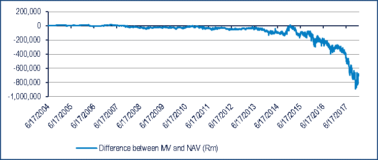
Remgro: chart reflecting estimated difference between the market value of Remgro and our calculation of its net asset value

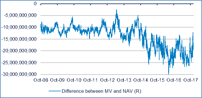
Source: Investec Wealth & Investment analyst model

Naspers: chart reflecting estimated difference between the market value of Naspers and our calculation of its net asset value

Source: Investec Wealth & Investment analyst model

Global savings and interest rates- will we see normalisation?

What the world needs now is more than love- there is also too little spending. [1]More of that would also be very welcome. Particularly welcome would be extra spending by business enterprises on capital equipment. This lack of demand, combined with a rising global savings rate, has created an abundance of saving that explains the exceptionally low interest rate rewards for saving in developed economies. This glut of savings followed the global financial crisis (GFC) of 2008-09 that made managers more fearful to spend or lend while additional regulations restricted their freedom to do so.

The story of the global glut of savings can be told in a few pictures provided by the World Bank shown below. When will then consider how the bond market in the US may be indicating some incipient revival of the animal spirits of US corporations. Encouraged, as they attest, by lower tax rates and much more sympathetic regulators.

Figure 1 charts gross global savings as a per cent of gross global incomes. (GNI) As may be seen share of savings of income has been rising steadily over the years. The GFC hit savings even harder than incomes (upon which savings depend) but since then savings have made an ever larger claim on incomes (26% in 2015). The global savings rate was only about 21% of incomes in the fast growing and higher interest rate world of the mid-nineties. It has been on a generally upward trend since, as may be seen.

Gross savings – (savings before amortisation of capital that turns gross into net savings) are dominated by the cash retained by corporations. Households may save – but other households over the same period may be large borrowers and reduce the net contribution households make to the capital market. And most governments are net borrowers- borrowing even more than they spend on infrastructure that is counted as saving.

Fig 1; Gross savings as per cent of Gross Global Income

As we show below in figure 2, the rate at which real capital – plant and infrastructure – has been accumulated has been trending in very much the opposite lower direction. There was a brief surge in the rate of capital formation in 2005 – a boom year for the global economy – but this was not sustained and was but 24% of global incomes in 2016- compared to a higher global savings rate of 26%.

Fig.2; Gross Capital Formation (% of GDP)

Source; World Bank

In the case of South Africa, with a lower gross savings rate of less than 18% of GDP, the cash retained by the corporate sector (including state owned enterprises) accounts for more than 100% of all gross savings. The household sector’s net contribution to gross savings flows is barely positive and the government sector is a net dis-saver. We show the trends in the SA savings rate below. The profits from the gold booms of the seventies and early eighties were responsible for the very high savings rates then.

Fig 3; South Africa – Gross Savings Rate

Source; World Bank

South Africa cannot realistically hope to raise its savings rate significantly. It can however hope to raise the rate at which capital expenditure is undertaken. That is by reducing the risks of investing in SA- and growing faster and attracting the savings to fund more rapid growth. That would be freely available from the large pool of global savings anxiously seeking better returns- given the right incentives and protections to do so. There is, as indicated, no global shortage of capital – only of attractive investment opportunities that SA could be offering.

The current rate of capital formation currently in SA is only slightly higher than the low savings rate – hence the small net inflows of foreign capital. The difference between any nation’s gross savings and capital formation is approximately equal to the net capital inflow and so the current account deficit on the balance of payments. The item that balances the current account deficit (exports-imports +debt service) – is the change in forex reserves- usually a comparatively small number.

South Africa could do with much faster growth that would encourage more capital formation and attract the foreign savings to fund this growth. And higher corporate incomes would mean more corporate savings. It is slow growth that is at the core of SA’s economic issues. Not the lack of savings. If we grew faster both the current account deficit and the capital inflows would be larger and the rate of capital formation higher. And a larger capital stock would bring more employment and higher incomes for a more productive labour force.

The US despite a relatively low and fairly stable savings rate (currently also around 18% of GNI as in South Africa) is, given the scale of its economy, still a large saver on the global stage. Though the US economy is the largest by far drawer on the global capital market to fund its spending as we show below in figure 8. While the US has been saving absolutely more recently, Chinese savings have now far overtaken US savings in absolute magnitude. Germany is another large saver, adding significantly to global savings in recent years, as we show below.

Fig. 4; Global Savings Rates

Source; World Bank

Fig.5; Gross savings (current US dollars) by economy

Source; World Bank

The Chinese are not only the largest contributor to global savings, saving an extraordinary 45% of their GNI – a rate that as may be seen has been declining from above 50%- they are also undertaking by far the largest share of global capital formation. They created plant and equipment – real capital – worth over USD 5 trillion in 2016 or at a rate equivalent to 45% of GNI, similar to the investment rate- meaning that most of the Chinese savings were utilised domestically.

Fig.6; China Gross Capital Formation (% GDP)

Source; World Bank

But this raises a very important issue for the Chinese. Given the rate at which they save and invest in real capital the realised growth in Chinese incomes must be regarded as disappointingly poor- even when about a 7 per cent p.a rate. It suggests that much of the capital formed is still unproductively utilised. The full discipline of western style capital markets is surely something still to be introduced to China to improve returns on savings. But for all the relative inefficiency of Chines capital, the sheer volume of Chinese capital formation has made it the dominant force in the market for minerals and metals that are used to create capital goods.

Fig.7; Gross capital formation by economy – current US dollars

Source; World Bank

In figure 8 below we show how The US dominates the demand side of the flows through global capital market- and the thrifty Europeans – the supply side. As may be seen these trends that made US economic actors the dominant utilisers of global capital are predominatly a post 2000 development.

It is these capital flows that drive the US dollar exchange rate – and by implication all other exchange rates. Trade flows react to exchange rates- rather than the other way round. This is also the case for SA. With one important difference- foreign trade for the US economy is equivalent to about 25% of GDP. In SA imports and exports – valued at unpredictable exchange rates are equal to about 50% of GDP.

Fig. 8, Net Financial Flows from Europe and to the US. Current US dollars

Source; World Bank

The flows of savings and flows into the US have not only moved the dollar they have moved interest rates. Perhaps the best measure of the global rewards for saving are found in the direction of the real rates of interest offered by an inflation linked bond issued by the US Treasury. Such a bond may be regarded as free of default as well as inflation risk. The risks of inflation are reflected in the yield on a vanilla bond. In the figure 9 below we compare the yield on a 10 Year US Treasury Bond and its inflation protected alternative with the same duration. As may be seen the nominal and real yields have both trended lower. The vanilla treasury bond was offering over 5% p.a in 2005- now the yield for a ten year loan provided the US is about 2.7% p.a. Real yields were over 2%. p.a. in 2005-06. They are now about a half of one per cent p.a. – after a period of negative returns in 2012-2013.

More important these yields have been rising in 2018 indicating some small degree of greater demands for capital. The real and nominal yields however remain very low by historic standards as will be appreciated. Normality – that is any sustained higher global growth rates, must mean much higher real yields. Higher nominal yields will also depend on how much inflation comes to be added to real yields.

Fig. 9; Nominal and Real 10 Year US Treasury Bond Yields (Daily Data 2005- 2018)

Source; Bloomberg and Investec Wealth and Investment

Fig. 10; Nominal and Real 10 Year US Treasury Bond Yields (Daily Data 2018)

Source; Bloomberg and Investec Wealth and Investment

In figure 11 below we show the difference between these nominal and real interest rates. These differences represent the extra compensation bond investors receive for taking on inflation risk. It may be regarded as a highly objective measure of inflationary expectations. The more inflation expected the wider must be the spread between nominal and real yields. As may be seen- excluding the impact of the GFC this spread or inflation expected has remained between two and three per cent per annum. It is important to recognise that these inflationary expectations remain very subdued despite a recent increase. Equity investors as well as bond investors must hope that inflation expectations remain subdued enough to hold down nominal interest rates even as real yields rise to reflect a stronger global economy and a revival of capital formation. Low inflation with faster growth is an especially favourable scenario for equity markets.

Fig.11; Inflation compensation in the US Treasury Bond Market – spread between nominal and real 10 year US Treasury Bond Yields

Source; Bloomberg and Investec Wealth and Investment

[1] With acknowledgement to Burt Bacharach

Lessons from US tax reforms

Taxes: Appearance and reality in the US and everywhere else

Reducing the US corporate tax rate and the taxes applied to offshore profits earned by US corporations and the repatriation of cash generated offshore, has had perhaps unintended consequences that are proving very helpful to the tax reformers. Some leading companies have immediately converted lower taxes to come into bonuses for their employees.

These reactions help raise the issue of who actually pays an income tax or a payroll tax. Those employees soon to notice a lower tax charge on their salary slips will have no doubts about who pays the income tax – and how they benefit from any reduction in tax rates. Shareholders receiving extra dividends, because the company has more after tax cash to distribute, will draw similar conclusions about the immediate benefits of lower tax rates.

But these immediate reactions to lower tax rates in the US will not be the last or the most important consequences of lower income tax rates. Lower tax rates will have improved the prospective returns on capital invested by US companies. More than pay dividends or buy back shares, the company may therefore wish to invest more in plant and equipment.

If so, and this seems very likely judged by the reactions of CEOs, the additional capacity will give these firms the capacity to produce more. To sell more they may well have to reduce prices or improve the other terms on which they supply their customers. The benefits of lower tax rates will thus also go to their customers in the form of lower prices or better quality or better service, depending on the competition to attract more custom. And workers may benefit as the firm hires more of them, perhaps on more favourable terms, again depending on the competition in the labour market for new hires.

In the long run the benefits of a higher return on shareholders capital, higher because less is paid away in taxes, will tend to be competed away. Actual returns after taxes may then fall away to a new equilibrium of lower required returns on a larger stock of equipment and a larger, better paid labour force in which more intellectual capital has been embedded. The effects of higher tax rates would similarly be reversed into higher prices as investment and hiring activity responds negatively to higher required returns before taxes.

These long run effects will be hard to identify, precisely because nothing much of what else will affect the economy will remain unchanged after a tax regime is changed and economic actors respond. Exchange rates may change, while tax rates in other countries may change to make imports more competitive. Trade across borders may be become more or less open. Yet it would be hard to argue that changes in taxes will not have wider consequences than is revealed on a payslip or dividend payment.

It is also surely true that the benefits, medical or pension etc. that employers provide for their workers will influence the supply of workers, skilled and unskilled, to the firm. The better the benefits, the greater will be the potential supply of job applicants and the lower the quit rates. Increased supplies of actual and potential workers in response to improved other benefits of employment will mean the firm has to offer less take home pay to attract the workers it wishes to hire.

Employees may well be paying for the benefits in the form of a cash salary sacrifice, which is to the advantage of the hiring firm. And taxpayers will be contributing, should the benefits in kind rather than cash enjoy much lower tax rates, in other forms of tax. Such tax favours for employees may help make the firm more competitive, in the form of a lower wage bill. This in turn may enable it to offer lower prices or better terms to their customers – as in the case of lower income taxes.
In these and many other ways, hard to identify, taxes tend to find their way into the prices consumers pay for the goods and services they buy. And this applies to all taxes and not only the VAT or sales taxes imposed on final expenditures.

Higher taxes mean higher prices and vice versa. And as important for the supply side effects of taxes of all kinds is how well the tax revenues are utilised. A good ratio between taxes collected and benefits provided, for obvious example in the quality of education supplied by governments, will tend to increase the supply of skills and lower costs of production and prices to the benefit of consumers ultimately.

The conclusion to come to when recognising the full ramifications of a tax system on the supply of and demand for goods and services, is to keep the tax system as simple as possible. That is to avoid trying to redistribute income through taxes of one kind or another (that find their way into prices) and hence may not redistribute income at all. All taxes may become a tax on expenditure rather than on income. Appearances of redistribution of income through can be very deceptive and damaging to an economy.

It would be more helpful to recognise reality and simply tax expenditure of all kinds at the same rate, thus avoiding income taxes, including taxes on income of companies and taxing one form of income in cash or kind at very different rates. Redistribution is best done by targeting government expenditure – not taxes. As is raising the taxes to pay for benefits as least disruptively as possible. 9 February 2018

A volatility storm – has it passed?

The S&P on Monday lost 4% by its close. The Dow had its largest one day loss in history, over 1000 points. In percentage terms it was the worst day for the New York markets since September 2011.

It is easier to understand what didn’t move the New York markets on Monday than what did. It was not any economic news, which was notably absent on the day. Nor was it interest rates. Interest rates moved the markets on Friday when they rose sharply in response to the impressive employment report. Both real and nominal bond yields closed sharply lower by the close on Monday and have maintained lower levels compared to Friday’s close on early Tuesday morning, even as the equity markets remained under pressure before the markets opened.

The most conspicuously unusual behaviour on markets was registered by the CBOE Volatility Index, the VIX. It closed 20 points higher at 37, the largest point and percentage change in this Index ever. And most of this increase took place in the last two hours of trading: it moved from 10 to over 30 in two hours. It appears that much of the price move and the huge volumes of trading activity associated with it was the result of special funds attempting to close out strategies based upon low volatility. Their attempts to do so forced up the Index and forced share prices lower.

The issue for market commentators before the market opened was how soon, as it is described, the systematic bid for volatility would subside. Judged by the strong recovery of the equity markets (S&P up one per cent as I write on Tuesday evening) in the first hour of trading the danger posed by rebalancing volatility strategies may have passed. Yet volatility – the form of minute to minute movements in share prices and Index averages of them – remains highly elevated. The VIX on 6 February continued to trade at these elevated levels as the market indices gyrate between positive and negative values.

Some economic realities

Perhaps in times when economic fundamentals appear irrelevant to company valuations, it is good to be reminded of just what has been happening at the economic coal face. Though coal is surely the wrong metaphor, the companies we refer to here are moving the frontier of economic activity – of how we work and consume that has changed so dramatically.

Some of the leading new economy companies reported their results for Q4 2017. The scale of their operations and the growth in their revenues is nothing less than very impressive. Apple for example reported quarterly sales of $88.29bn, up 13% on the same quarter in 2016. Amazon reported Q4 sales of $60.5bn, up no less than 38% on the same quarter a year before and up 31% for the year. Facebook grew sales in Q4 2017 to $12.97bn and by 47% and Alphabet generated revenues in Q4 of $32.32bn, up 24%. And Microsoft (in business for much longer) grew its sales in Q4 2017 by 12%, to $25.83bn.

All these companies that are thriving impressively and are being generously valued accordingly – described as the FAAGMS – have a competitive and a regulatory threat. Their success to date is as vulnerable to disruption by competitors – known and unknown – as they have proved to be to what were then established ways of doing business.

However their success and the market dominance it seems to create – of which their approving customers are the arbiters – is bound to attract the attention of regulators and tax collectors. That is of economic agents, with interests and powers of their own, who are philosophically unwilling to concede the race for dominance in a market place is to be determined by consumers and regulate accordingly. They would do well to accept that what constitutes the relevant market place is fluid and incapable of being usefully defined and confined. Competition for the budgets of households and of all the firms that ultimately compete for their favour remains highly intense, as the fast growing sales of the Apples, Amazons, Facebooks, Googles and Microsofts prove. Society should best leave the unpredictable outcomes to this competition. 7 February

Equity markets and interest rates in the US

Equity markets and interest rates in the US – will we avoid inflation surprises?

The equity markets in the US have had an outstanding run. The S&P 500 is up 26% since January 2017 and has advanced with unusually low volatility. Day to day movements in the Index have been very limited by the standards of the past. The fundamentals of the market have been supportive of higher valuations. High operating margins and rising earnings, with upward revisions of earnings to come, combined with still low interest rates, have attracted these higher valuations. The future of earnings and margins has been further enhanced by the income tax cuts for corporates, small businesses and individuals. The animal spirits of corporate leaders are stirring, promising a boost to the economy from a strong pick up in capital expenditure.

The concern is that unexpectedly higher interest rates can offset these benefits, as earnings are discounted to estimate present values. As we show below, US Treasury bond market yields have been rising this year – but from abnormally low levels. Nominal yields for 10-year money have increased this year from 2.45% to current levels of 2.72%. So have real yields – they have risen from a very low half a per cent in early 2018 to over 0.6% now. Furthermore, the gap between nominal and real inflation protected interest rates has increased from 2.45% at the start of 2018 to the current level of over 2.7%. This spread reveals the inflation rate predicted by the bond market. The bond market is anticipating and being compensated for slightly more inflation expected over the next 10 years.

The Fed’s target for inflation is 2% – a target that it is still to meet and is by no means certain of meeting any time soon. The Federal Open Market Committee, reporting this week (31 January 2018) still expects inflation to stabilise around its 2% objective over the medium term in its latest statement. It also repeated its view “that near-term risks to the economic outlook appear roughly balanced, but the Committee is monitoring inflation developments closely…”

The most supportive scenario for the equity market will be one of rising real interest rates – indicating stronger growth in demands for capital – coupled with still very subdued expected inflation that will sustain low nominal interest rates. It is not higher real interest rates that represent danger to equity valuations. It is more inflation expected that would drive nominal interest rates higher that represent the threat to equity markets. Not only the Fed, but the markets, will be watching inflation developments closely. They will also be watching each other closely to avoid inflation surprises. Equity investors must hope that inflation does not surprise on the high side. Low inflation and strong real growth are what equity markets will thrive on, as they have done lately. 2 February 2018